PS3.17

The information in this publication was considered technically sound by the consensus of persons engaged in the development and approval of the document at the time it was developed. Consensus does not necessarily mean that there is unanimous agreement among every person participating in the development of this document.

NEMA standards and guideline publications, of which the document contained herein is one, are developed through a voluntary consensus standards development process. This process brings together volunteers and/or seeks out the views of persons who have an interest in the topic covered by this publication. While NEMA administers the process and establishes rules to promote fairness in the development of consensus, it does not write the document and it does not independently test, evaluate, or verify the accuracy or completeness of any information or the soundness of any judgments contained in its standards and guideline publications.

NEMA disclaims liability for any personal injury, property, or other damages of any nature whatsoever, whether special, indirect, consequential, or compensatory, directly or indirectly resulting from the publication, use of, application, or reliance on this document. NEMA disclaims and makes no guaranty or warranty, expressed or implied, as to the accuracy or completeness of any information published herein, and disclaims and makes no warranty that the information in this document will fulfill any of your particular purposes or needs. NEMA does not undertake to guarantee the performance of any individual manufacturer or seller's products or services by virtue of this standard or guide.

In publishing and making this document available, NEMA is not undertaking to render professional or other services for or on behalf of any person or entity, nor is NEMA undertaking to perform any duty owed by any person or entity to someone else. Anyone using this document should rely on his or her own independent judgment or, as appropriate, seek the advice of a competent professional in determining the exercise of reasonable care in any given circumstances. Information and other standards on the topic covered by this publication may be available from other sources, which the user may wish to consult for additional views or information not covered by this publication.

NEMA has no power, nor does it undertake to police or enforce compliance with the contents of this document. NEMA does not certify, test, or inspect products, designs, or installations for safety or health purposes. Any certification or other statement of compliance with any health or safety-related information in this document shall not be attributable to NEMA and is solely the responsibility of the certifier or maker of the statement.

Foreword

This DICOM Standard was developed according to the procedures of the DICOM Standards Committee.

The DICOM Standard is structured as a multi-part document using the guidelines established in [ISO/IEC Directives, Part 2].

PS3.1 should be used as the base reference for the current parts of this standard.

1 Scope and Field of Application

This part of the DICOM Standard contains explanatory information in the form of Normative and Informative Annexes.

2 Normative References

The following standards contain provisions which, through reference in this text, constitute provisions of this Standard. At the time of publication, the editions indicated were valid. All standards are subject to revision, and parties to agreements based on this Standard are encouraged to investigate the possibilities of applying the most recent editions of the standards indicated below.

2.1 International Organization for Standardization (ISO) and International Electrotechnical Commission (IEC)

[ISO/IEC Directives, Part 2] ISO/IEC. 2016/05. 7.0. Rules for the structure and drafting of International Standards. http://www.iec.ch/members_experts/refdocs/iec/isoiecdir-2%7Bed7.0%7Den.pdf .

3 Definitions

For the purposes of this Standard the following definitions apply.

4 Symbols and Abbreviations

The following symbols and abbreviations are used in this Part of the Standard.

FHIR: HL7 Fast Healthcare Interoperability Resources (draft standard)

5 Conventions

Terms listed in Section 3 are capitalized throughout the document.

A Explanation of Patient Orientation (Normative)

This Annex was formerly located in Annex E “Explanation of Patient Orientation (Normative)” in PS3.3 in the 2003 and earlier revisions of the standard.

This Annex provides an explanation of how to use the patient orientation data elements.

Figure A-1. Standard Anatomic Position Directions - Whole Body

Figure A-2. Standard Anatomic Position Directions - Hand

Figure A-3. Standard Anatomic Position Directions - Foot

As for the hand, the direction labels are based on the foot in the standard anatomic position. For the right foot, for example, RIGHT will be in the direction of the 5th toe. This assignment will remain constant through movement or positioning of the extremity. This is also true of the HEAD and FOOT directions.

Figure A-4. Views - Anterior and Lateral

Figure A-5. Planes - Whole Body - Transverse

Figure A-6. Planes - Whole Body - Sagittal

Figure A-7. Planes - Whole Body - Coronal

Figure A-8. Planes - Hand

Figure A-9. Planes - Double Obliquity

Figure A-10. Standard Anatomic Position Directions - Paired Hands

Figure A-11. Breast - MedioLateral Oblique

Figure A-12. Panoramic Zonogram Directions

B Integration of Modality Worklist and Modality Performed Procedure Step in The Original DICOM Standard (Informative)

This Annex was formerly located in Annex G “Integration of Modality Worklist and Modality Performed Procedure Step in the Original DICOM Standard (Informative)” in PS3.3 in the 2003 and earlier revisions of the standard.

DICOM was published in 1993 and effectively addresses image communication for a number of modalities and Image Management functions for a significant part of the field of medical imaging. Since then, many additional medical imaging specialties have contributed to the extension of the DICOM Standard and developed additional Image Object Definitions. Furthermore, there have been discussions about the harmonization of the DICOM Real-World domain model with other standardization bodies. This effort has resulted in a number of extensions to the DICOM Standard. The integration of the Modality Worklist and Modality Performed Procedure Step address an important part of the domain area that was not included initially in the DICOM Standard. At the same time, the Modality Worklist and Modality Performed Procedure Step integration make steps in the direction of harmonization with other standardization bodies (CEN TC 251, HL7, etc.).

The purpose of this Annex is to show how the original DICOM Standard relates to the extension for Modality Worklist Management and Modality Performed Procedure Step. The two included figures outline the void filled by the Modality Worklist Management and Modality Performed Procedure Step specification, and the relationship between the original DICOM Data Model and the extended model.

Figure B-1. Functional View - Modality Worklist and Modality Performed Procedure Step Management in the Context of DICOM Service Classes

The management of a patient starts when the patient enters a physical facility (e.g., a hospital, a clinic, an imaging center) or even before that time. The DICOM Patient Management SOP Class provides many of the functions that are of interest to imaging departments. Figure B-1 is an example where one presumes that an order for a procedure has been issued for a patient. The order for an imaging procedure results in the creation of a Study Instance within the DICOM Study Management SOP Class. At the same time (A) the Modality Worklist Management SOP Class enables a modality operator to request the scheduling information for the ordered procedures. A worklist can be constructed based on the scheduling information. The handling of the requested imaging procedure in DICOM Study Management and in DICOM Worklist Management are closely related. The worklist also conveys patient/study demographic information that can be incorporated into the images.

Worklist Management is completed once the imaging procedure has started and the Scheduled Procedure Step has been removed from the Worklist, possibly in response to the Modality Performed Procedure Step (B). However, Study Management continues throughout all stages of the Study, including interpretation. The actual procedure performed (based on the request) and information about the images produced are conveyed by the DICOM Study Component SOP Class or the Modality Performed Procedure Step SOP Classes.

Figure B-2. Relationship of the Original Model and the Extensions for Modality Worklist and Modality Performed Procedure Step Management

Figure B-2 shows the relationship between the original DICOM Real-World model and the extensions of this Real-World model required to support the Modality Worklist and the Modality Performed Procedure Step. The new parts of the model add entities that are needed to request, schedule, and describe the performance of imaging procedures, concepts that were not supported in the original model. The entities required for representing the Worklist form a natural extension of the original DICOM Real-World model.

Common to both the original model and the extended model is the Patient entity. The Service Episode is an administrative concept that has been shown in the extended model in order to pave the way for future adaptation to a common model supported by other standardization groups including HL7, CEN TC 251 WG 3, CAP-IEC, etc. The Visit is in the original model but not shown in the extended model because it is a part of the Service Episode.

There is a 1 to 1 relationship between a Requested Procedure and the DICOM Study (A). A DICOM Study is the result of a single Requested Procedure. A Requested Procedure can result in only one Study.

A n:m relationship exists between a Scheduled Procedure Step and a Modality Performed Procedure Step (B). The concept of a Modality Performed Procedure Step is a superset of the Study Component concept contained in the original DICOM model. The Modality Performed Procedure Step SOP Classes provide a means to relate Modality Performed Procedure Steps to Scheduled Procedure Steps.

C Waveforms (Informative)

This Annex was formerly located in Annex J “Waveforms (Informative)” in PS3.3 in the 2003 and earlier revisions of the standard.

C.1 Domain of Application

Waveform acquisition is part of both the medical imaging environment and the general clinical environment. Because of its broad use, there has been significant previous and complementary work in waveform standardization of which the following are particularly important:

ASTM E31.16 - E1467: Specification for Transferring Digital Neurophysiological Data Between Independent Computer Systems
CEN TC251 PT5-007 - prENV1064 draft: Standard Communications Protocol for Computer-Assisted Electrocardiography (SCP-ECG).
CEN TC251 PT5-021 - draft: Vital Signs Information Representation Standard (VITAL)
HL7 Automated Data SIG: HL7 Version 2.3, Chapter 7.14-20
IEEE P1073 - draft: Medical Information Bus Standard (MIB)
DICOM Section A.10 in PS3.3: Standalone Curve Information Object Definition

For DICOM, the domain of waveform standardization is waveform acquisition within the imaging context. It is specifically meant to address waveform acquisitions that will be analyzed with other data that is transferred and managed using the DICOM protocol. It allows the addition of waveform data to that context with minimal incremental cost. Further, it leverages the DICOM persistent object capability for maintaining referential relationships to other data collected in a multi-modality environment, including references necessary for multi-modality synchronization.

Waveform interchange in other clinical contexts may use different protocols more appropriate to those domains. In particular, HL7 may be used for transfer of waveform observations to general clinical information systems, and MIB may be used for real-time physiological monitoring and therapy.

The waveform information object definition in DICOM has been specifically harmonized at the semantic level with the HL7 waveform message format. The use of a common object model allows straightforward transcoding and interoperation between systems that use DICOM for waveform interchange and those that use HL7, and may be viewed as an example of common semantics implemented in the differing syntaxes of two messaging systems.

Note

HL7 allows transport of DICOM SOP Instances (information objects) encapsulated within HL7 messages. Since the DICOM and HL7 waveform semantics are harmonized, DICOM Waveform SOP Instances need not be transported as encapsulated data, as they can be transcoded to native HL7 Waveform Observation format.

C.2 Use Cases

The following are specific use case examples for waveforms in the imaging environment.

Case 1: Catheterization Laboratory - During a cardiac catheterization, several independent pieces of data acquisition equipment may be brought together for the exam. An electrocardiographic subsystem records surface ECG waveforms; an X-ray angiographic subsystem records motion images; a hemodynamic subsystem records intracardiac pressures from a sensor on the catheter. These subsystems send their acquired data by network to a repository. These data are assembled at an analytic workstation by retrieving from the repository. For a left ventriculographic procedure, the ECG is used by the physician to determine the time of maximum and minimum ventricular fill, and when coordinated with the angiographic images, an accurate estimate of the ejection fraction can be calculated. For a valvuloplasty procedure, the hemodynamic waveforms are used to calculate the pre-intervention and post-intervention pressure gradients.
Case 2: Electrophysiology Laboratory - An electrophysiological exam will capture waveforms from multiple sensors on a catheter; the placement of the catheter in the heart is captured on an angiographic image. At an analytic workstation, the exact location of the sensors can thus be aligned with a model of the heart, and the relative timing of the arrival of the electrophysiological waves at different cardiac locations can be mapped.
Case 3: Stress Exam - A stress exam may involve the acquisition of both ECG waveforms and echocardiographic ultrasound images from portable equipment at different stages of the test. The waveforms and the echocardiograms are output on an interchange disk, which is then input and read at a review station. The physician analyzes both types of data to make a diagnosis of cardiac health.

C.3 Time Synchronization Frame of Reference

Synchronization of acquisition across multiple modalities in a single study (e.g., angiography and electrocardiography) requires either a shared trigger, or a shared clock. A Synchronization Module within the Frame of Reference Information Entity specifies the synchronization mechanism. A common temporal environment used by multiple equipment is identified by a shared Synchronization Frame of Reference UID. How this UID is determined and distributed to the participating equipment is outside the scope of the standard.

The method used for time synchronization of equipment clocks is implementation or site specific, and therefore outside the scope of this proposal. If required, standard time distribution protocols are available (e.g., NTP, IRIG, GPS).

An informative description of time distribution methods can be found at: http://www.bancomm.com/cntpApp.htm

A second method of synchronizing acquisitions is to utilize a common reference channel (temporal fiducial), which is recorded in the data acquired from the several equipment units participating in a study, and/or that is used to trigger synchronized data acquisitions. For instance, the "X-ray on" pulse train that triggers the acquisition of frames for an X-ray angiographic SOP Instance can be recorded as a waveform channel in a simultaneously acquired hemodynamic waveform SOP Instance, and can be used to align the different object instances. Associated with this Supplement are proposed coded entry channel identifiers to specifically support this synchronization mechanism (DICOM Terminology Mapping Resource Context Group ID 3090).

C.4 Waveform Acquisition Model

Figure C.4-1 shows a canonical model of waveform data acquisition. A patient is the subject of the study. There may be several sensors placed at different locations on or in the patient, and waveforms are measurements of some physical quality (metric) by those sensors (e.g., electrical voltage, pressure, gas concentration, or sound). The sensor is typically connected to an amplifier and filter, and its output is sampled at constant time intervals and digitized. In most cases, several signal channels are acquired synchronously. The measured signal usually originates in the anatomy of the patient, but an important special case is a signal that originates in the equipment, either as a stimulus, such as a cardiac pacing signal, as a therapy, such as a radio frequency signal used for ablation, or as a synchronization signal.

Figure C.4-1. Waveform Acquisition Model

C.5 Waveform Information Model

The part of the composite information object that carries the waveform data is the Waveform Information Entity (IE). The Waveform IE includes the technical parameters of waveform acquisition and the waveform samples.

The information model, or internal organizational structure, of the Waveform IE is shown in Figure C.5-1. A waveform information object includes data from a continuous time period during which signals were acquired. The object may contain several multiplex groups, each defined by digitization with the same clock whose frequency is defined for the group. Within each multiplex group there will be one or more channels, each with a full technical definition. Finally, each channel has its set of digital waveform samples.

Figure C.5-1. DICOM Waveform Information Model

C.6 Harmonization With HL7

This Waveform IE definition is harmonized with the HL7 waveform semantic constructs, including the channel definition attributes and the use of multiplex groups for synchronously acquired channels. The use of a common object model allows straightforward transcoding and interoperation between systems that use DICOM for waveform interchange and those that use HL7, and may be viewed as an example of common semantics implemented in the differing syntaxes of two messaging systems.

This section describes the congruence between the DICOM Waveform IE and the HL7 version 2.3 waveform message format (see HL7 version 2.3 Chapter 7, sections 7.14 - 7.20).

C.6.1 HL7 Waveform Observation

Waveforms in HL7 messages are sent in a set of OBX (Observation) Segments. Four subtypes of OBX segments are defined:

The CHN subtype defines one channel in a CD (Channel Definition) Data Type
The TIM subtype defines the start time of the waveform data in a TS (Time String) Data Type
The WAV subtype carries the waveform data in an NA (Numeric Array) or MA (Multiplexed Array) Data Type (ASCII encoded samples, character delimited)
The ANO subtype carries an annotation in a CE (Coded Entry) Data Type with a reference to a specific time within the waveform to which the annotation applies

Other segments of the HL7 message definition specify patient and study identification, whose harmonization with DICOM constructs is not defined in this Annex.

C.6.2 Channel Definition

The Waveform Module Channel Definition sequence attribute (003A,0200) is defined in harmonization with the HL7 Channel Definition (CD) Data Type, in accordance with the following Table. Each Item in the Channel Definition sequence attribute corresponds to an OBX Segment of subtype CHN.

Table C.6-1. Correspondence Between DICOM and HL7 Channel Definition

DICOM Attribute	DICOM Tag	HL7 CD Data Type Component
Waveform Channel Number	(003A,0202)	Channel Identifier (number&name)
Channel Label	(003A,0203)	Channel Identifier (number&name)
Channel Source Sequence	(003A,0208)	Waveform Source
Channel Source Modifier Sequence	(003A,0209)	Waveform Source
Channel Sensitivity	(003A,0210)	Channel Sensitivity and Units
Channel Sensitivity Units Sequence	(003A,0211)	Channel Sensitivity and Units
Channel Sensitivity Correction Factor	(003A,0212)	Channel Calibration Parameters (correctionfactor&baseline&timeskew)
Channel Baseline	(003A,0213)
Channel Time Skew	(003A,0214)
[Group] Sampling Frequency	(003A,001A)	Channel Sampling Frequency
Channel Minimum Value	(5400,0110)	Minimum and Maximum Data Values (minimum & maximum)
Channel Maximum Value	(5400,0112)	Minimum and Maximum Data Values (minimum & maximum)
Channel Offset	(003A,0218)	not defined in HL7
Channel Status	(003A,0205)
Filter Low Frequency	(003A,0220)
Filter High Frequency	(003A,0221)
Notch Filter Frequency	(003A,0222)
Notch Filter Bandwidth	(003A,0223)

In the DICOM information object definition, the sampling frequency is defined for the multiplex group, while in HL7 it is defined for each channel, but is required to be identical for all multiplexed channels.

Note that in the HL7 syntax, Waveform Source is a string, rather than a coded entry as used in DICOM. This should be considered in any transcoding between the two formats.

C.6.3 Timing

In HL7, the exact start time for waveform data is sent in an OBX Segment of subtype TIM. The corresponding DICOM attributes, which must be combined to form the equivalent time string, are:

Acquisition DateTime	(0008,002A)
Multiplex Group Time Offset	(0018,1068)

C.6.4 Waveform Data

The DICOM binary encoding of data samples in the Waveform Data attribute (5400,1010) corresponds to the ASCII representation of data samples in the HL7 OBX Segment of subtype WAV. The same channel-interleaved multiplexing used in the HL7 MA (Multiplexed Array) Data Type is used in the DICOM Waveform Data attribute.

Because of its binary representation, DICOM uses several data elements to specify the precise encoding, as listed in the following Table. There are no corresponding HL7 data elements, since HL7 uses explicit character-delimited ASCII encoding of data samples.

Number of Waveform Channels	(003A,0005)
Number of Waveform Samples	(003A,0010)
Waveform Bits Stored	(003A,021A)
Waveform Bits Allocated	(5400,1004)
Waveform Sample Interpretation	(5400,1006)
Waveform Padding Value	(5400,100A)

C.6.5 Annotation

In HL7, Waveform Annotation is sent in an OBX Segment of subtype ANO, using the CE (Coded Entry) Data Type CE. This corresponds precisely to the DICOM Annotation using Coded Entry Sequences. However, HL7 annotation ROI is to a single point only (time reference), while DICOM allows reference to ranges of samples delimited by time or by explicit sample position.

C.7 Harmonization With SCP-ECG

The SCP-ECG standard is designed for recording routine resting electrocardiograms. Such ECGs are reviewed prior to cardiac imaging procedures, and a typical use case would be for SCP-ECG waveforms to be translated to DICOM for inclusion with the full cardiac imaging patient record.

SCP-ECG provides for either simultaneous or non-simultaneous recording of the channels, but does not provide a multiplexed data format (each channel is separately encoded). When translating to DICOM, each subset of simultaneously recorded channels may be encoded in a Waveform Sequence Item (multiplex group), and the delay to the recording of each multiplex group shall be encoded in the Multiplex Group Time Offset (0018,1068).

The electrode configuration of SCP-ECG Section 1 may be translated to the DICOM Acquisition Context (0040,0555) sequence items using TID 3401 “ECG Acquisition Context” and Context Groups 3263 and 3264.

The lead identification of SCP-ECG Section 3, a term coded as an unsigned integer, may be translated to the DICOM Waveform Channel Source (003A,0208) coded sequence using CID 3001 “ECG Leads”.

Pacemaker spike records of SCP-ECG Section 7 may be translated to items in the Waveform Annotations Sequence (0040,B020) with a code term from CID 3335 “ECG Annotations”. The annotation sequence item may record the spike amplitude in its Numeric Value and Measurement Units attributes.

D SR Encoding Example (Informative)

This Annex was formerly located in Annex K “SR Encoding Example (Informative)” in PS3.3 in the 2003 and earlier revisions of the standard.

The following is a simple and non-comprehensive illustration of the encoding of the Informative SR Content Tree Example in PS3.3.

SR Tree Depth	Nesting	Attribute	Tag	VR	VL (hex)	Value
		SOP Class UID	(0008,0016)	UI	001e	1.2.840.10008.5.1.4.1.1.88.33
		SOP Instance UID	(0008,0018)	UI	0012	1.2.3.4.5.6.7.300
		Study Date	(0008,0020)	DA	0008	19991029
		Content Date	(0008,0023)	DA	0008	19991029
		Study Time	(0008,0030)	TM	0006	154500
		Content Time	(0008,0033)	TM	0006	154510
		Accession Number	(0008,0050)	SH	0006	123456
		Modality	(0008,0060)	CS	0002	SR
		Manufacturer	(0008,0070)	LO	0004	WG6
		Referring Physician's Name	(0008,0090)	PN	0014	Luke^Will^^Dr.^M.D.
		Coding Scheme Identification Sequence	(0008,0110)	SQ	ffffffff
	%item
	>	Coding Scheme Designator	(0008,0102)	SH	000e	99STElsewhere
	>	Coding Scheme UID	(0008,010C)	UI	0010	1.2.3.4.6.7.8.91
	>	Responsible Organization	(0008,0116)	ST	0034	Informatics Dept St Elsewhere Hosp Boston, MA 02390
	%enditem
	%endseq
		Referenced Performed Procedure Step Sequence	(0008,1111)	SQ	ffffffff
	%endseq
		Patient's Name	(0010,0010)	PN	000e	Homer^Jane^^^
		Patient's ID	(0010,0020)	LO	0006	234567
		Patient's Birth Date	(0010,0030)	DA	0008	19991109
		Patient's Sex	(0010,0040)	CS	0002	F
		Study Instance UID	(0020,000D)	UI	0012	1.2.3.4.5.6.7.100
		Series Instance UID	(0020,000E)	UI	0012	1.2.3.4.5.6.7.200
		Study ID	(0020,0010)	SH	0006	345678
		Series Number	(0020,0011)	IS	0002	1
		Instance (formerly Image) Number	(0020,0013)	IS	0002	1
1		Value Type	(0040,a040)	CS	000a	CONTAINER
1		Concept Name Code Sequence	(0040,a043)	SQ	ffffffff
1	%item
1	>	Code Value	(0008,0100)	SH	0006	43468-8
1	>	Coding Scheme Designator	(0008,0102)	SH	0002	LN
1	>	Code Meaning	(0008,0104)	LO	000c	X-Ray Report
1	%enditem
	%endseq
1		Continuity Of Content	(0040,a050)	CS	0008	SEPARATE
		Verifying Observer Sequence	(0040,a073)	SQ	ffffffff
	%item
	>	Verifying Organization	(0040,a027)	LO	0004	WG6
	>	Verification DateTime	(0040,a030)	DT	000e	19991029154510
	>	Verifying Observer Name	(0040,a075)	PN	000e	Jones^Joe^^Dr^
	>	Verifying Observer Identification Code Sequence	(0040,a088)	SQ	ffffffff
	%item
	>>	Code Value	(0008,0100)	SH	0006	369842
	>>	Coding Scheme Designator	(0008,0102)	SH	000e	99STElsewhere
	>>	Code Meaning	(0008,0104)	LO	0006	369842
	%enditem
	%endseq
	%enditem
	%endseq
		Referenced Request Sequence	(0040,a370)	SQ	ffffffff
	%item
	>	Accession Number	(0008,0050)	SH	0006	123456
	>	Referenced Study Sequence	(0008,1110)	SQ	ffffffff
	%endseq
	>	Study Instance UID	(0020,000D)	UI	0012	1.2.3.4.5.6.7.100
	>	Requested Procedure Description	(0032,1060)	LO	000a	Chest Xray
	>	Requested Procedure Code Sequence	(0032,1064)	SQ	ffffffff
	%item
	>>	Code Value	(0008,0100)	SH	0006	42272-5
	>>	Coding Scheme Designator	(0008,0102)	SH	0002	LN
	>>	Code Meaning	(0008,0104)	LO	001a	Chest X-Ray PA and lateral
	%enditem
	%endseq
	>	Requested Procedure ID	(0040,1001)	SH	0006	012340
	>	Placer Order Number/Imaging Service Request	(0040,2016)	LO	0
	>	Filler Order Number/Imaging Service Request	(0040,2017)	LO	0
	%enditem
	%endseq
		Performed Procedure Code Sequence	(0040,a372)	SQ	ffffffff
	%item
	>	Code Value	(0008,0100)	SH	0006	42272-5
	>	Coding Scheme Designator	(0008,0102)	SH	0002	LN
	>	Code Meaning	(0008,0104)	LO	001a	Chest X-Ray PA and lateral
	%enditem
	%endseq
		Current Requested Procedure Evidence Sequence	(0040,a375)	SQ	ffffffff
	%item
	>	Referenced Series Sequence	(0008,1115)	SQ	ffffffff
	%item
	>>	Referenced SOP Sequence	(0008,1199)	SQ	ffffffff
	%item
	>>>	Referenced SOP Class UID	(0008,1150)	UI	0008	1.2.3.4
	>>>	Referenced SOP Instance UID	(0008,1155)	UI	000a	1.2.3.4.5
	%enditem
	%endseq
	>>	Series Instance UID	(0020,000E)	UI	0012	1.2.3.4.5.6.7.200
	%enditem
	%endseq
	>	Study Instance UID	(0020,000D)	UI	0012	1.2.3.4.5.6.7.100
	%enditem
	%endseq
		Completion Flag	(0040,a491)	CS	0008	COMPLETE
		Verification Flag	(0040,a493)	CS	0008	VERIFIED
1		Content Sequence	(0040,a730)	SQ	ffffffff
1.1	%item
1.1	>	Relationship Type	(0040,a010)	CS	0010	HAS OBS CONTEXT
1.1	>	Value Type	(0040,a040)	CS	0006	PNAME
1.1	>	Concept Name Code Sequence	(0040,a043)	SQ	ffffffff
1.1	%item
1.1	>>	Code Value	(0008,0100)	SH	0006	121008
1.1	>>	Coding Scheme Designator	(0008,0102)	SH	0004	DCM
1.1	>>	Code Meaning	(0008,0104)	LO	0014	Person Observer Name
1.1	%enditem
1.1	%endseq
1.1	>	Person Name	(0040,a123)	PN	0010	Smith^John^^Dr^
1.1	%enditem
1.2	%item
1.2	>	Relationship Type	(0040,a010)	CS	0010	HAS OBS CONTEXT
1.2	>	Value Type	(0040,a040)	CS	0006	UIDREF
1.2	>	Concept Name Code Sequence	(0040,a043)	SQ	ffffffff
1.2	%item
1.2	>>	Code Value	(0008,0100)	SH	0006	121018
1.2	>>	Coding Scheme Designator	(0008,0102)	SH	0004	DCM
1.2	>>	Code Meaning	(0008,0104)	LO	001c	Procedure Study Instance UID
1.2	%enditem
1.2	%endseq
1.2	>	UID	(0040,a124)	UI	0012	1.2.3.4.5.6.7.100
1.2	%enditem
1.3	%item
1.3	>	Relationship Type	(0040,a010)	CS	0010	HAS OBS CONTEXT
1.3	>	Value Type	(0040,a040)	CS	0006	PNAME
1.3	>	Concept Name Code Sequence	(0040,a043)	SQ	ffffffff
1.3	%item
1.3	>>	Code Value	(0008,0100)	SH	0006	121029
1.3	>>	Coding Scheme Designator	(0008,0102)	SH	0004	DCM
1.3	>>	Code Meaning	(0008,0104)	LO	000c	Subject Name
1.3	%enditem
1.3	%endseq
1.3	>	Person Name	(0040,a123)	PN	000e	Homer^Jane^^^
1.3	%enditem
1.4	%item
1.4	>	Relationship Type	(0040,a010)	CS	0008	CONTAINS
1.4	>	Value Type	(0040,a040)	CS	0004	CODE
1.4	>	Concept Name Code Sequence	(0040,a043)	SQ	ffffffff
1.4	%item
1.4	>>	Code Value	(0008,0100)	SH	0006	121071
1.4	>>	Coding Scheme Designator	(0008,0102)	SH	0004	DCM
1.4	>>	Code Meaning	(0008,0104)	LO	0008	Finding
1.4	%enditem
1.4	%endseq
1.4	>	Concept Code Sequence	(0040,a168)	SQ	ffffffff
1.4	%item
1.4	>>	Code Value	(0008,0100)	SH	0006	G-D701
1.4	>>	Coding Scheme Designator	(0008,0102)	SH	0004	SRT
1.4	>>	Code Meaning	(0008,0104)	LO	0004	Mass
1.4	%enditem
1.4	%endseq
1.4	>	Content Sequence	(0040,a730)	SQ	ffffffff
1.4.1	%item
1.4.1	>>	Relationship Type	(0040,a010)	CS	000e	HAS PROPERTIES
1.4.1	>>	Value Type	(0040,a040)	CS	0004	NUM
1.4.1	>>	Concept Name Code Sequence	(0040,a043)	SQ	ffffffff
1.4.1	%item
1.4.1	>>>	Code Value	(0008,0100)	SH	0006	M-02550
1.4.1	>>>	Coding Scheme Designator	(0008,0102)	SH	0004	SRT
1.4.1	>>>	Code Meaning	(0008,0104)	LO	0008	Diameter
1.4.1	%enditem
1.4.1	%endseq
1.4.1	>>	Measured Value Sequence	(0040,a300)	SQ	ffffffff
1.4.1	%item
1.4.1	>>>	Measurement Units Code Sequence	(0040,08ea)	SQ	ffffffff
1.4.1	%item
1.4.1	>>>>	Code Value	(0008,0100)	SH	0002	cm
1.4.1	>>>>	Coding Scheme Designator	(0008,0102)	SH	0004	UCUM
1.4.1	>>>>	Code Meaning	(0008,0104)	LO	0002	cm
1.4.1	%enditem
1.4.1	%endseq
1.4.1	>>>	Numeric Value	(0040,a30a)	DS	0004	1.3
1.4.1	%enditem
1.4.1	%endseq
1.4.1	%enditem
1.4.2	%item
1.4.2	>>	Relationship Type	(0040,a010)	CS	000e	HAS PROPERTIES
1.4.2	>>	Value Type	(0040,a040)	CS	0004	CODE
1.4.2	>>	Concept Name Code Sequence	(0040,a043)	SQ	ffffffff
1.4.2	%item
1.4.2	>>>	Code Value	(0008,0100)	SH	0006	G-A428
1.4.2	>>>	Coding Scheme Designator	(0008,0102)	SH	0004	SRT
1.4.2	>>>	Code Meaning	(0008,0104)	LO	0006	Margin
1.4.2	%enditem
1.4.2	%endseq
1.4.2	>>	Concept Code Sequence	(0040,a168)	SQ	ffffffff
1.4.2	%item
1.4.2	>>>	Code Value	(0008,0100)	SH	0006	112136
1.4.2	>>>	Coding Scheme Designator	(0008,0102)	SH	0004	DCM
1.4.2	>>>	Code Meaning	(0008,0104)	LO	000a	Spiculated
1.4.2	%enditem
1.4.2	%endseq
1.4.2	%enditem
1.4	%endseq
1.4	%enditem
1.5	%item
1.5	>	Referenced SOP Sequence	(0008,1199)	SQ	ffffffff
1.5	%item
1.5	>>	Referenced SOP Class UID	(0008,1150)	UI	0008	1.2.3.4
1.5	>>	Referenced SOP Instance UID	(0008,1155)	UI	000a	1.2.3.4.5
1.5	%enditem
1.5	%endseq
1.5	>	Relationship Type	(0040,a010)	CS	0008	CONTAINS
1.5	>	Value Type	(0040,a040)	CS	0006	IMAGE
1.5	>	Concept Name Code Sequence	(0040,a043)	SQ	ffffffff
1.5	%item
1.5	>>	Code Value	(0008,0100)	SH	0006	121079
1.5	>>	Coding Scheme Designator	(0008,0102)	SH	0004	DCM
1.5	>>	Code Meaning	(0008,0104)	LO	0008	Baseline
1.5	%enditem
1.5	%endseq
1.5	%enditem
1.6	%item
1.6	>	Relationship Type	(0040,a010)	CS	0008	CONTAINS
1.6	>	Value Type	(0040,a040)	CS	000a	CONTAINER
1.6	>	Concept Name Code Sequence	(0040,a043)	SQ	ffffffff
1.6	%item
1.6	>>	Code Value	(0008,0100)	SH	0006	55110-1
1.6	>>	Coding Scheme Designator	(0008,0102)	SH	0002	LN
1.6	>>	Code Meaning	(0008,0104)	LO	000c	Conclusions
1.6	%enditem
1.6	%endseq
1.6		Continuity Of Content	(0040,a050)	CS	0008	SEPARATE
1.6	>	Content Sequence	(0040,a730)	SQ	ffffffff
1.6.1	%item
1.6.1	>>	Relationship Type	(0040,a010)	CS	0008	CONTAINS
1.6.1	>>	Value Type	(0040,a040)	CS	0004	CODE
1.6.1	>>	Concept Name Code Sequence	(0040,a043)	SQ	ffffffff
1.6.1	%item
1.6.1	>>>	Code Value	(0008,0100)	SH	0006	121077
1.6.1	>>>	Coding Scheme Designator	(0008,0102)	SH	0004	DCM
1.6.1	>>>	Code Meaning	(0008,0104)	LO	000a	Conclusion
1.6.1	%enditem
1.6.1	%endseq
1.6.1	>>	Concept Code Sequence	(0040,a168)	SQ	ffffffff
1.6.1	%item
1.6.1	>>>	Code Value	(0008,0100)	SH	0006	888000
1.6.1	>>>	Coding Scheme Designator	(0008,0102)	SH	000e	99STElsewhere
1.6.1	>>>	Code Meaning	(0008,0104)	LO	0014	Probable malignancy
1.6.1	%enditem
1.6.1	%endseq
1.6.1	>>	Content Sequence	(0040,a730)	SQ	ffffffff
1.6.1.1	%item
1.6.1.1	>>>	Relationship Type	(0040,a010)	CS	000e	INFERRED FROM
1.6.1.1	>>>	Referenced Content Item Identifier	(0040,db73)	UL	000c	0001,0004,0002
1.6.1.1	%enditem
1.6.1.2	%item
1.6.1.2	>>>	Relationship Type	(0040,a010)	CS	000e	INFERRED FROM
1.6.1.2	>>>	Referenced Content Item Identifier	(0040,db73)	UL	000c	0001,0007,0001
1.6.1.2	%enditem
1.6.1	%endseq
1.6.1	%enditem
1.6	%endseq
1.6	%enditem
1.7	%item
1.7	>	Relationship Type	(0040,a010)	CS	0008	CONTAINS
1.7	>	Value Type	(0040,a040)	CS	000a	CONTAINER
1.7	>	Concept Name Code Sequence	(0040,a043)	SQ	ffffffff
1.7	%item
1.7	>>	Code Value	(0008,0100)	SH	0006	59776-5
1.7	>>	Coding Scheme Designator	(0008,0102)	SH	0006	LN
1.7	>>	Code Meaning	(0008,0104)	LO	0008	Findings
1.7	%enditem
1.7	%endseq
1.7		Continuity Of Content	(0040,a050)	CS	0008	SEPARATE
1.7	>	Content Sequence	(0040,a730)	SQ	ffffffff
1.7.1	%item
1.7.1	>>	Relationship Type	(0040,a010)	CS	0008	CONTAINS
1.7.1	>>	Value Type	(0040,a040)	CS	0006	SCOORD
1.7.1	>>	Concept Name Code Sequence	(0040,a043)	SQ	ffffffff
1.7.1	%item
1.7.1	>>>	Code Value	(0008,0100)	SH	0006	121080
1.7.1	>>>	Coding Scheme Designator	(0008,0102)	SH	0004	DCM
1.7.1	>>>	Code Meaning	(0008,0104)	LO	001c	Best illustration of finding
1.7.1	%enditem
1.7.1	%endseq
1.7.1	>>	Content Sequence	(0040,a730)	SQ	ffffffff
1.7.1.1	%item
1.7.1.1	>>>	Referenced SOP Sequence	(0008,1199)	SQ	ffffffff
1.7.1.1	%item
1.7.1.1	>>>>	Referenced SOP Class UID	(0008,1150)	UI	0008	1.2.3.4
1.7.1.1	>>>>	Referenced SOP Instance UID	(0008,1155)	UI	000a	1.2.3.4.6
1.7.1.1	%enditem
1.7.1.1	%endseq
1.7.1.1	>>>	Relationship Type	(0040,a010)	CS	000e	SELECTED FROM
1.7.1.1	>>>	Value Type	(0040,a040)	CS	0006	IMAGE
1.7.1.1	%enditem
1.7.1	%endseq
1.7.1	>>	Graphic Data	(0070,0022)	FL	0020	0,0,0,0,0,0,0,0
1.7.1	>>	Graphic Type	(0070,0023)	CS	0008	POLYLINE
1.7.1	%enditem
1.7	%endseq
1.7	%enditem
1.8	%item
1.8	>	Relationship Type	(0040,a010)	CS	0010	HAS CONCEPT MOD
1.8	>	Value Type	(0040,a040)	CS	0004	CODE
1.8	>	Concept Name Code Sequence	(0040,a043)	SQ	ffffffff
1.8	%item
1.8	>>	Code Value	(0008,0100)	SH	000a	LP28726-5
1.8	>>	Coding Scheme Designator	(0008,0102)	SH	0002	LN
1.8	>>	Code Meaning	(0008,0104)	LO	0006	Views
1.8	%enditem
1.8	%endseq
1.8	>	Concept Code Sequence	(0040,a168)	SQ	ffffffff
1.8	%item
1.8	>>	Code Value	(0008,0100)	SH	000a	LP33431-5
1.8	>>	Coding Scheme Designator	(0008,0102)	SH	0002	LN
1.8	>>	Code Meaning	(0008,0104)	LO	000e	PA and Lateral
1.8	%enditem
1.8	%endseq
1.8	%enditem
1	%endseq

E Mammography CAD (Informative)

This Annex was formerly located in Annex L “Mammography CAD (Informative)” in PS3.3 in the 2003 and earlier revisions of the standard.

E.1 Mammography CAD SR Content Tree Structure

The templates for the Mammography CAD SR IOD are defined in Mammography CAD SR IOD Templates in PS3.16 . Relationships defined in the Mammography CAD SR IOD templates are by-value, unless otherwise stated. Content items referenced from another SR object instance, such as a prior Mammography CAD SR, are inserted by-value in the new SR object instance, with appropriate original source observation context. It is necessary to update Rendering Intent, and referenced content item identifiers for by-reference relationships, within content items paraphrased from another source.

Figure E.1-1. Top Levels of Mammography CAD SR Content Tree

The Document Root, Image Library, Summaries of Detections and Analyses, and CAD Processing and Findings Summary sub-trees together form the content tree of the Mammography CAD SR IOD. There are no constraints regarding the 1-n multiplicity of the Individual Impression/Recommendation or its underlying structure, other than the TID 4001 “Mammography CAD Overall Impression/Recommendation” and TID 4003 “Mammography CAD Individual Impression/Recommendation” requirements in PS3.16. Individual Impression/Recommendation containers may be organized, for example per image, per finding or composite feature, or some combination thereof.

Figure E.1-2. Summary of Detections and Analyses Levels of Mammography CAD SR Content Tree

The Summary of Detections and Summary of Analyses sub-trees identify the algorithms used and the work done by the CAD device, and whether or not each process was performed on one or more entire images or selected regions of images. The findings of the detections and analyses are not encoded in the summary sub-trees, but rather in the CAD Processing and Findings Summary sub-tree. CAD processing may produce no findings, in which case the sub-trees of the CAD Processing and Findings Summary sub-tree are incompletely populated. This occurs in the following situations:

All algorithms succeeded, but no findings resulted
Some algorithms succeeded, some failed, but no findings resulted
All algorithms failed

Note

If the tree contains no Individual Impression/Recommendation nodes and all attempted detections and analyses succeeded then the mammography CAD device made no findings.
Detections and Analyses that are not attempted are not listed in the Summary of Detections and Summary of Analyses trees.
If the code value of the Summary of Detections or Summary of Analyses codes in TID 4000 “Mammography CAD Document Root” is "Not Attempted" then no detail is provided as to which algorithms were not attempted.

Figure E.1-3. Example of Individual Impression/Recommendation Levels of Mammography CAD SR Content Tree

The shaded area in Figure E.1-3 demarcates information resulting from Detection, whereas the unshaded area is information resulting from Analysis. This distinction is used in determining whether to place algorithm identification information in the Summary of Detections or Summary of Analyses sub-trees.

The clustering of calcifications within a single image is considered to be a Detection process that results in a Single Image Finding. The spatial correlation of a calcification cluster in two views, resulting in a Composite Feature, is considered Analysis. The clustering of calcifications in a single image is the only circumstance in which a Single Image Finding can result from the combination of other Single Image Findings, which must be Individual Calcifications.

Once a Single Image Finding or Composite Feature has been instantiated, it may be referenced by any number of Composite Features higher in the tree.

E.2 Mammography CAD SR Observation Context Encoding

Any content item in the Content tree that has been inserted (i.e., duplicated) from another SR object instance has a HAS OBS CONTEXT relationship to one or more content items that describe the context of the SR object instance from which it originated. This mechanism may be used to combine reports (e.g., Mammography CAD 1, Mammography CAD 2, Human).
By-reference relationships within Single Image Findings and Composite Features paraphrased from prior Mammography CAD SR objects need to be updated to properly reference Image Library Entries carried from the prior object to their new positions in the present object.

The Impression/Recommendation section of the SR Document Content tree of a Mammography CAD SR IOD may contain a mixture of current and prior single image findings and composite features. The content items from current and prior contexts are target content items that have a by-value INFERRED FROM relationship to a Composite Feature content item. Content items that come from a context other than the Initial Observation Context have a HAS OBS CONTEXT relationship to target content items that describe the context of the source document.

In Figure E.2-1, Composite Feature and Single Image Finding are current, and Single Image Finding (from Prior) is duplicated from a prior document.

Figure E.2-1. Example of Use of Observation Context

E.3 Mammography CAD SR Examples

The following is a simple and non-comprehensive illustration of an encoding of the Mammography CAD SR IOD for Mammography computer aided detection results. For brevity, some Mandatory content items are not included, such as several acquisition context content items for the images in the Image Library.

E.3.1 Example 1: Calcification and Mass Detection With No Findings

A mammography CAD device processes a typical screening mammography case, i.e., there are four films and no cancer. Mammography CAD runs both density and calcification detection successfully and finds nothing. The mammograms resemble:

Figure E.3-1. Mammograms as Described in Example 1

The content tree structure would resemble:

Node	Code Meaning of Concept Name	Code Meaning or Example Value	TID
1	Mammography CAD Report		TID 4000
1.1	Image Library		TID 4000
1.1.1		IMAGE 1	TID 4020
1.1.1.1	Image Laterality	Right	TID 4020
1.1.1.2	Image View	Cranio-caudal	TID 4020
1.1.1.3	Study Date	19980101	TID 4020
1.1.2		IMAGE 2	TID 4020
1.1.2.1	Image Laterality	Left	TID 4020
1.1.2.2	Image View	Cranio-caudal	TID 4020
1.1.2.3	Study Date	19980101	TID 4020
1.1.3		IMAGE 3	TID 4020
1.1.3.1	Image Laterality	Right	TID 4020
1.1.3.2	Image View	Medio-lateral oblique	TID 4020
1.1.3.3	Study Date	19980101	TID 4020
1.1.4		IMAGE 4	TID 4020
1.1.4.1	Image Laterality	Left	TID 4020
1.1.4.2	Image View	Medio-lateral oblique	TID 4020
1.1.4.3	Study Date	19980101	TID 4020
1.2	CAD Processing and Findings Summary	All algorithms succeeded; without findings	TID 4001
1.3	Summary of Detections	Succeeded	TID 4000
1.3.1	Successful Detections		TID 4015
1.3.1.1	Detection Performed	Mammography breast density	TID 4017
1.3.1.1.1	Algorithm Name	"Density Detector"	TID 4019
1.3.1.1.2	Algorithm Version	"V3.7"	TID 4019
1.3.1.1.3		Reference to node 1.1.1	TID 4017
1.3.1.1.4		Reference to node 1.1.2	TID 4017
1.3.1.1.5		Reference to node 1.1.3	TID 4017
1.3.1.1.6		Reference to node 1.1.4	TID 4017
1.3.1.2	Detection Performed	Individual Calcification	TID 4017
1.3.1.2.1	Algorithm Name	"Calc Detector"	TID 4019
1.3.1.2.2	Algorithm Version	"V2.4"	TID 4019
1.3.1.2.3		Reference to node 1.1.1	TID 4017
1.3.1.2.4		Reference to node 1.1.2	TID 4017
1.3.1.2.5		Reference to node 1.1.3	TID 4017
1.3.1.2.6		Reference to node 1.1.4	TID 4017
1.4	Summary of Analyses	Not Attempted	TID 4000

E.3.2 Example 2: Calcification and Mass Detection With Findings

A mammography CAD device processes a screening mammography case with four films and a mass in the left breast. Mammography CAD runs both density and calcification detection successfully. It finds two densities in the LCC, one density in the LMLO, a cluster of two calcifications in the RCC and a cluster of 20 calcifications in the RMLO. It performs two clustering algorithms. One identifies individual calcifications and then clusters them, and the second simply detects calcification clusters. It performs mass correlation and combines one of the LCC densities and the LMLO density into a mass; the other LCC density is flagged Not for Presentation, therefore not intended for display to the end-user. The mammograms resemble:

Figure E.3-2. Mammograms as Described in Example 2

The content tree structure in this example is complex. Structural illustrations of portions of the content tree are placed within the content tree table to show the relationships of data within the tree. Some content items are duplicated (and shown in boldface) to facilitate use of the diagrams.

Figure E.3-3. Content Tree Root of Example 2 Content Tree

Node	Code Meaning of Concept Name	Code Meaning or Example Value	TID
1	Mammography CAD Report		TID 4000
1.1	Image Library		TID 4000
1.2	CAD Processing and Findings Summary	All algorithms succeeded; with findings	TID 4001
1.3	Summary of Detections	Succeeded	TID 4000
1.4	Summary of Analyses	Succeeded	TID 4000

Figure E.3-4. Image Library Branch of Example 2 Content Tree

Node	Code Meaning of Concept Name	Code Meaning or Example Value	TID
1.1	Image Library		TID 4000
1.1.1		IMAGE 1	TID 4020
1.1.1.1	Image Laterality	Right	TID 4020
1.1.1.2	Image View	Cranio-caudal	TID 4020
1.1.1.3	Study Date	19990101	TID 4020
1.1.2		IMAGE 2	TID 4020
1.1.2.1	Image Laterality	Left	TID 4020
1.1.2.2	Image View	Cranio-caudal	TID 4020
1.1.2.3	Study Date	19990101	TID 4020
1.1.3		IMAGE 3	TID 4020
1.1.3.1	Image Laterality	Right	TID 4020
1.1.3.2	Image View	Medio-lateral oblique	TID 4020
1.1.3.3	Study Date	19990101	TID 4020
1.1.4		IMAGE 4	TID 4020
1.1.4.1	Image Laterality	Left	TID 4020
1.1.4.2	Image View	Medio-lateral oblique	TID 4020
1.1.4.3	Study Date	19990101	TID 4020

Figure E.3-5. CAD Processing and Findings Summary Bifurcation of Example 2 Content Tree

Node	Code Meaning of Concept Name	Code Meaning or Example Value	TID
1.2	CAD Processing and Findings Summary	All algorithms succeeded; with findings	TID 4001
1.2.1	Individual Impression/Recommendation		TID 4003
1.2.2	Individual Impression/Recommendation		TID 4003
1.2.3	Individual Impression/Recommendation		TID 4003
1.2.4	Individual Impression/Recommendation		TID 4003

Figure E.3-6. Individual Impression/Recommendation 1.2.1 from Example 2 Content Tree

Node	Code Meaning of Concept Name	Code Meaning or Example Value	TID
1.2.1	Individual Impression/Recommendation		TID 4003
1.2.1.1	Rendering Intent	Presentation Required	TID 4003
1.2.1.2	Composite Feature	Mass	TID 4004
1.2.1.2.1	Rendering Intent	Presentation Required	TID 4004
1.2.1.2.2	Composite type	Target content items are related spatially	TID 4005
1.2.1.2.3	Scope of Feature	Feature was detected on multiple images	TID 4005
1.2.1.2.4	Algorithm Name	"Mass Maker"	TID 4019
1.2.1.2.5	Algorithm Version	"V1.9"	TID 4019
1.2.1.2.6	Single Image Finding	Mammography breast density	TID 4006
1.2.1.2.7	Single Image Finding	Mammography breast density	TID 4006

Figure E.3-7. Single Image Finding Density 1.2.1.2.6 from Example 2 Content Tree

Node	Code Meaning of Concept Name	Code Meaning or Example Value	TID
1.2.1.2.6	Single Image Finding	Mammography breast density	TID 4006
1.2.1.2.6.1	Rendering Intent	Presentation Required	TID 4006
1.2.1.2.6.2	Algorithm Name	"Density Detector"	TID 4019
1.2.1.2.6.3	Algorithm Version	"V3.7"	TID 4019
1.2.1.2.6.4	Center	POINT	TID 4021
1.2.1.2.6.4.1		Reference to node 1.1.2	TID 4021
1.2.1.2.6.5	Outline	SCOORD	TID 4021
1.2.1.2.6.5.1		Reference to node 1.1.2	TID 4021

Figure E.3-8. Single Image Finding Density 1.2.1.2.7 from Example 2 Content Tree

Node	Code Meaning of Concept Name	Code Meaning or Example Value	TID
1.2.1.2.7	Single Image Finding	Mammography breast density	TID 4006
1.2.1.2.7.1	Rendering Intent	Presentation Required	TID 4006
1.2.1.2.7.2	Algorithm Name	"Density Detector"	TID 4019
1.2.1.2.7.3	Algorithm Version	"V3.7"	TID 4019
1.2.1.2.7.4	Center	POINT	TID 4021
1.2.1.2.7.4.1		Reference to node 1.1.4	TID 4021
1.2.1.2.7.5	Outline	SCOORD	TID 4021
1.2.1.2.7.5.1		Reference to node 1.1.4	TID 4021
1.2.1.2.7.6	Area of Defined Region	1 cm²	TID 1401
1.2.1.2.7.6.1	Area Outline	SCOORD	TID 1401
1.2.1.2.7.6.1.1		Reference to node 1.1.4	TID 1401

Figure E.3-9. Individual Impression/Recommendation 1.2.2 from Example 2 Content Tree

Node	Code Meaning of Concept Name	Code Meaning or Example Value	TID
1.2.2	Individual Impression/Recommendation		TID 4003
1.2.2.1	Rendering Intent	Not for Presentation	TID 4003
1.2.2.2	Single Image Finding	Mammography breast density	TID 4006
1.2.2.2.1	Rendering Intent	Not for Presentation	TID 4006
1.2.2.2.2	Algorithm Name	"Density Detector"	TID 4019
1.2.2.2.3	Algorithm Version	"V3.7"	TID 4019
1.2.2.2.4	Center	POINT	TID 4021
1.2.2.2.4.1		Reference to node 1.1.2	TID 4021
1.2.2.2.5	Outline	SCOORD	TID 4021
1.2.2.2.5.1		Reference to node 1.1.2	TID 4021

Figure E.3-10. Individual Impression/Recommendation 1.2.3 from Example 2 Content Tree

Node	Code Meaning of Concept Name	Code Meaning or Example Value	TID
1.2.3	Individual Impression/Recommendation		TID 4003
1.2.3.1	Rendering Intent	Presentation Required	TID 4003
1.2.3.2	Single Image Finding	Calcification Cluster	TID 4006
1.2.3.2.1	Rendering Intent	Presentation Required	TID 4006
1.2.3.2.2	Algorithm Name	"Calc Cluster Detector"	TID 4019
1.2.3.2.3	Algorithm Version	"V2.4"	TID 4019
1.2.3.2.4	Center	POINT	TID 4021
1.2.3.2.4.1		Reference to node 1.1.3	TID 4021
1.2.3.2.5	Outline	SCOORD	TID 4021
1.2.3.2.5.1		Reference to node 1.1.3	TID 4021
1.2.3.2.6	Number of Calcifications	20	TID 4010

Figure E.3-11. Individual Impression/Recommendation 1.2.4 from Example 2 Content Tree

Node	Code Meaning of Concept Name	Code Meaning or Example Value	TID
1.2.4	Individual Impression/Recommendation		TID 4003
1.2.4.1	Rendering Intent	Presentation Required	TID 4003
1.2.4.2	Single Image Finding	Calcification Cluster	TID 4006
1.2.4.2.1	Rendering Intent	Presentation Required	TID 4006
1.2.4.2.2	Algorithm Name	"Calc Clustering"	TID 4019
1.2.4.2.3	Algorithm Version	"V2.4"	TID 4019
1.2.4.2.4	Center	POINT	TID 4021
1.2.4.2.4.1		Reference to node 1.1.1	TID 4021
1.2.4.2.5	Outline	SCOORD	TID 4021
1.2.4.2.5.1		Reference to node 1.1.1	TID 4021
1.2.4.2.6	Number of Calcifications	2	TID 4010

Figure E.3-12. Single Image Finding 1.2.4.2.7 from Example 2 Content Tree

Node	Code Meaning of Concept Name	Code Meaning or Example Value	TID
1.2.4.2.7	Single Image Finding	Individual Calcification	TID 4006
1.2.4.2.7.1	Rendering Intent	Presentation Optional	TID 4006
1.2.4.2.7.2	Algorithm Name	"Calc Detector"	TID 4019
1.2.4.2.7.3	Algorithm Version	"V2.4"	TID 4019
1.2.4.2.7.4	Center	POINT	TID 4021
1.2.4.2.7.4.1		Reference to node 1.1.1	TID 4021
1.2.4.2.7.5	Outline	SCOORD	TID 4021
1.2.4.2.7.5.1		Reference to node 1.1.1	TID 4021

Figure E.3-13. Single Image Finding 1.2.4.2.8 from Example 2 Content Tree

Node	Code Meaning of Concept Name	Code Meaning or Example Value	TID
1.2.4.2.8	Single Image Finding	Individual Calcification	TID 4006
1.2.4.2.8.1	Rendering Intent	Presentation Optional	TID 4006
1.2.4.2.8.2	Algorithm Name	"Calc Detector"	TID 4019
1.2.4.2.8.3	Algorithm Version	"V2.4"	TID 4019
1.2.4.2.8.4	Center	POINT	TID 4021
1.2.4.2.8.4.1		Reference to node 1.1.1	TID 4021
1.2.4.2.8.5	Outline	SCOORD	TID 4021
1.2.4.2.8.5.1		Reference to node 1.1.1	TID 4021

Figure E.3-14. Summary of Detections Branch of Example 2 Content Tree

Node	Code Meaning of Concept Name	Code Meaning or Example Value	TID
1.3	Summary of Detections	Succeeded	TID 4000
1.3.1	Successful Detections		TID 4015
1.3.1.1	Detection Performed	Mammography breast density	TID 4017
1.3.1.1.1	Algorithm Name	"Density Detector"	TID 4019
1.3.1.1.2	Algorithm Version	"V3.7"	TID 4019
1.3.1.1.3		Reference to node 1.1.1	TID 4017
1.3.1.1.4		Reference to node 1.1.2	TID 4017
1.3.1.1.5		Reference to node 1.1.3	TID 4017
1.3.1.1.6		Reference to node 1.1.4	TID 4017
1.3.1.2	Detection Performed	Individual Calcification	TID 4017
1.3.1.2.1	Algorithm Name	"Calc Detector"	TID 4019
1.3.1.2.2	Algorithm Version	"V2.4"	TID 4019
1.3.1.2.3		Reference to node 1.1.1	TID 4017
1.3.1.2.4		Reference to node 1.1.2	TID 4017
1.3.1.2.5		Reference to node 1.1.3	TID 4017
1.3.1.2.6		Reference to node 1.1.4	TID 4017
1.3.1.3	Detection Performed	Calcification Cluster	TID 4017
1.3.1.3.1	Algorithm Name	"Calc Clustering"	TID 4019
1.3.1.3.2	Algorithm Version	"V2.4"	TID 4019
1.3.1.3.3		Reference to node 1.1.1	TID 4017
1.3.1.4	Detection Performed	Calcification Cluster	TID 4017
1.3.1.4.1	Algorithm Name	"Calc Cluster Detector"	TID 4019
1.3.1.4.2	Algorithm Version	"V2.4"	TID 4019
1.3.1.4.3		Reference to node 1.1.1	TID 4017
1.3.1.4.4		Reference to node 1.1.2	TID 4017
1.3.1.4.5		Reference to node 1.1.3	TID 4017
1.3.1.4.6		Reference to node 1.1.4	TID 4017

Figure E.3-15. Summary of Analyses Branch of Example 2 Content Tree

Node	Code Meaning of Concept Name	Code Meaning or Example Value	TID
1.4	Summary of Analyses	Succeeded	TID 4000
1.4.1	Successful Analyses		TID 4016
1.4.1.1	Analysis Performed	Mass Correlation	TID 4018
1.4.1.1.1	Algorithm Name	"Mass Maker"	TID 4019
1.4.1.1.2	Algorithm Version	"V1.9"	TID 4019
1.4.1.1.3		Reference to node 1.1.2	TID 4018
1.4.1.1.4		Reference to node 1.1.4	TID 4018

E.3.3 Example 3: Calcification and Mass Detection, Temporal Differencing With Findings

The patient in Example 2 returns for another mammogram. A more comprehensive mammography CAD device processes the current mammogram; analyses are performed that determine some content items for Overall and Individual Impression/Recommendations. Portions of the prior mammography CAD report (Example 2) are incorporated into this report. In the current mammogram the number of calcifications in the RCC has increased, and the size of the mass in the left breast has increased from 1 to 4 cm².

Figure E.3-16. Mammograms as Described in Example 3

Italicized entries (xxx) in the following table denote references to or by-value inclusion of content tree items reused from the prior Mammography CAD SR instance (Example 2).

Node	Code Meaning of Concept Name	Code Meaning or Example Value	TID
1	Mammography CAD Report		TID 4000

While the Image Library contains references to content tree items reused from the prior Mammography CAD SR instance, the images are actually used in the mammography CAD analysis and are therefore not italicized as indicated above.

Node	Code Meaning of Concept Name	Code Meaning or Example Value	TID
1.1	Image Library		TID 4000
1.1.1		IMAGE 1	TID 4020
1.1.1.1	Image Laterality	Right	TID 4020
1.1.1.2	Image View	Cranio-caudal	TID 4020
1.1.1.3	Study Date	20000101	TID 4020
1.1.2		IMAGE 2	TID 4020
1.1.2.1	Image Laterality	Left	TID 4020
1.1.2.2	Image View	Cranio-caudal	TID 4020
1.1.2.3	Study Date	20000101	TID 4020
1.1.3		IMAGE 3	TID 4020
1.1.3.1	Image Laterality	Right	TID 4020
1.1.3.2	Image View	Medio-lateral oblique	TID 4020
1.1.3.3	Study Date	20000101	TID 4020
1.1.4		IMAGE 4	TID 4020
1.1.4.1	Image Laterality	Left	TID 4020
1.1.4.2	Image View	Medio-lateral oblique	TID 4020
1.1.4.3	Study Date	20000101	TID 4020
1.1.5		IMAGE 5	TID 4020
1.1.5.1	Image Laterality	Right	TID 4020
1.1.5.2	Image View	Cranio-caudal	TID 4020
1.1.5.3	Study Date	19990101	TID 4020
1.1.6		IMAGE 6	TID 4020
1.1.6.1	Image Laterality	Left	TID 4020
1.1.6.2	Image View	Cranio-caudal	TID 4020
1.1.6.3	Study Date	19990101	TID 4020
1.1.7		IMAGE 7	TID 4020
1.1.7.1	Image Laterality	Right	TID 4020
1.1.7.2	Image View	Medio-lateral oblique	TID 4020
1.1.7.3	Study Date	19990101	TID 4020
1.1.8		IMAGE 8	TID 4020
1.1.8.1	Image Laterality	Left	TID 4020
1.1.8.2	Image View	Medio-lateral oblique	TID 4020
1.1.8.3	Study Date	19990101	TID 4020

Current year content:

Node	Code Meaning of Concept Name	Code Meaning or Example Value	TID
1.2	CAD Processing and Findings Summary	All algorithms succeeded; with findings	TID 4001
1.2.1	Assessment Category	4 - Suspicious abnormality, biopsy should be considered	TID 4002
1.2.2	Recommend Follow-up Interval	0 days	TID 4002
1.2.3	Algorithm Name	"Mammogram Analyzer"	TID 4019
1.2.4	Algorithm Version	"V1.0"	TID 4019
1.2.5	Individual Impression/Recommendation		TID 4003
1.2.5.1	Rendering Intent	Presentation Required	TID 4003
1.2.5.2	Differential Diagnosis/Impression	Increase in size	TID 4002
1.2.5.3	Impression Description	"Worrisome increase in size"	TID 4002
1.2.5.4	Recommended Follow-up	Needle localization and biopsy	TID 4002
1.2.5.5	Certainty of impression	84%	TID 4002
1.2.5.6	Algorithm Name	"Lesion Analyzer"	TID 4019
1.2.5.7	Algorithm Version	"V1.0"	TID 4019
1.2.5.8	Composite Feature	Mass	TID 4004
1.2.5.8.1	Rendering Intent	Presentation Required	TID 4004
1.2.5.8.2	Composite type	Target content items are related temporally	TID 4005
1.2.5.8.3	Scope of Feature	Feature was detected on multiple images	TID 4005
1.2.5.8.4	Algorithm Name	"Temporal Change"	TID 4019
1.2.5.8.5	Algorithm Version	"V0.1"	TID 4019
1.2.5.8.6	Certainty of Feature	91%	TID 4005
1.2.5.8.7	Probability of Cancer	84%	TID 4005
1.2.5.8.8	Pathology	Invasive lobular carcinoma	TID 4005
1.2.5.8.9	Difference in Size	3 cm²	TID 4005
1.2.5.8.9.1		Reference to node 1.2.5.8.13.7.6	TID 4005
1.2.5.8.9.2		Reference to node 1.2.5.8.14.8.6	TID 4005
1.2.5.8.10	Lesion Density	High density	TID 4005
1.2.5.8.11	Shape	Lobular	TID 4005
1.2.5.8.12	Margins	Microlobulated	TID 4005
1.2.5.8.13	Composite Feature	Mass	TID 4004
1.2.5.8.13.1	Rendering Intent	Presentation Required	TID 4004
1.2.5.8.13.2	Composite type	Target content items are related spatially	TID 4005
1.2.5.8.13.3	Scope of Feature	Feature was detected on multiple images	TID 4005
1.2.5.8.13.4	Algorithm Name	"Mass Maker"	TID 4019
1.2.5.8.13.5	Algorithm Version	"V1.9"	TID 4019
1.2.5.8.13.6	Single Image Finding	Mammography breast density	TID 4006
1.2.5.8.13.6.1	Rendering Intent	Presentation Required	TID 4006
1.2.5.8.13.6.2	Algorithm Name	"Density Detector"	TID 4019
1.2.5.8.13.6.3	Algorithm Version	"V3.7"	TID 4019
1.2.5.8.13.6.4	Center	POINT	TID 4021
1.2.5.8.13.6.4.1		Reference to node 1.1.2	TID 4021
1.2.5.8.13.6.5	Outline	SCOORD	TID 4021
1.2.5.8.13.6.5.1		Reference to node 1.1.2	TID 4021
1.2.5.8.13.7	Single Image Finding	Mammography breast density	TID 4006
1.2.5.8.13.7.1	Rendering Intent	Presentation Required	TID 4006
1.2.5.8.13.7.2	Algorithm Name	"Density Detector"	TID 4019
1.2.5.8.13.7.3	Algorithm Version	"V3.7"	TID 4019
1.2.5.8.13.7.4	Center	POINT	TID 4021
1.2.5.8.13.7.4.1		Reference to node 1.1.4	TID 4021
1.2.5.8.13.7.5	Outline	SCOORD	TID 4021
1.2.5.8.13.7.5.1		Reference to node 1.1.4	TID 4021
1.2.5.8.13.7.6	Area of Defined Region	4 cm²	TID 1401
1.2.5.8.13.7.6.1	Area Outline	SCOORD	TID 1401
1.2.5.8.13.7.6. 1.1		Reference to node 1.1.4	TID 1401

Included content from prior mammography CAD report (see Example 2, starting with node 1.2.1.2)

Node	Code Meaning of Concept Name	Code Meaning or Example Value	TID
1.2.5.8.14	Composite Feature	Mass	TID 4004
1.2.5.8.14.1	Rendering Intent	Presentation Required	TID 4004
1.2.5.8.14.2	Composite type	Target content items are related spatially	TID 4005
1.2.5.8.14.3	Scope of Feature	Feature was detected on multiple images	TID 4005
1.2.5.8.14.4	Algorithm Name	"Mass Maker"	TID 4019
1.2.5.8.14.5	Algorithm Version	"V1.9"	TID 4019
1.2.5.8.14.6	[Observation Context content items]		TID 4022
1.2.5.8.14.7	Single Image Finding	Mammography breast density	TID 4006
1.2.5.8.14.7.1	Rendering Intent	Presentation Required	TID 4006
1.2.5.8.14.7.2	Algorithm Name	"Density Detector"	TID 4019
1.2.5.8.14.7.3	Algorithm Version	"V3.7"	TID 4019
1.2.5.8.14.7.4	Center	POINT	TID 4021
1.2.5.8.14.7.4.1		Reference to node 1.1.6	TID 4021
1.2.5.8.14.7.5	Outline	SCOORD	TID 4021
1.2.5.8.14.7.5.1		Reference to node 1.1.6	TID 4021
1.2.5.8.14.8	Single Image Finding	Mammography breast density	TID 4006
1.2.5.8.14.8.1	Rendering Intent	Presentation Required	TID 4006
1.2.5.8.14.8.2	Algorithm Name	"Density Detector"	TID 4019
1.2.5.8.14.8.3	Algorithm Version	"V3.7"	TID 4019
1.2.5.8.14.8.4	Center	POINT	TID 4021
1.2.5.8.14.8.4.1		Reference to node 1.1.8	TID 4021
1.2.5.8.14.8.5	Outline	SCOORD	TID 4021
1.2.5.8.14.8.5.1		Reference to node 1.1.8	TID 4021
1.2.5.8.14.8.6	Area of Defined Region	1 cm²	TID 1401
1.2.5.8.14.8.6.1	Area Outline	SCOORD	TID 1401
1.2.5.8.14.8.6.1.1		Reference to node 1.1.8	TID 1401

Node	Code Meaning of Concept Name	Code Meaning or Example Value	TID
1.2.6	Individual Impression/Recommendation		TID 4003
1.2.6.1	Rendering Intent	Not for Presentation	TID 4003
1.2.6.2	Single Image Finding	Mammography breast density	TID 4006
1.2.6.2.1	Rendering Intent	Not for Presentation	TID 4006
1.2.6.2.2	Algorithm Name	"Density Detector"	TID 4019
1.2.6.2.3	Algorithm Version	"V3.7"	TID 4019
1.2.6.2.4	Center	POINT	TID 4021
1.2.6.2.4.1		Reference to node 1.1.2	TID 4021
1.2.6.2.5	Outline	SCOORD	TID 4021
1.2.6.2.5.1		Reference to node 1.1.2	TID 4021
1.2.7	Individual Impression/Recommendation	INDIVIDUAL	TID 4003
1.2.7.1	Rendering Intent	Presentation Required	TID 4003
1.2.7.2	Single Image Finding	Calcification Cluster	TID 4006
1.2.7.2.1	Rendering Intent	Presentation Required	TID 4006
1.2.7.2.2	Algorithm Name	"Calc Cluster Detector"	TID 4019
1.2.7.2.3	Algorithm Version	"V2.4"	TID 4019
1.2.7.2.4	Center	POINT	TID 4021
1.2.7.2.4.1		Reference to node 1.1.3	TID 4021
1.2.7.2.5	Outline	SCOORD	TID 4021
1.2.7.2.5.1		Reference to node 1.1.3	TID 4021
1.2.7.2.6	Number of Calcifications	20	TID 4010
1.2.8	Individual Impression/Recommendation		TID 4003
1.2.8.1	Rendering Intent	Presentation Required	TID 4003
1.2.8.2	Differential Diagnosis/Impression	Increase in number of calcifications	TID 4002
1.2.8.3	Impression Description	"Calcification cluster has increased in size"	TID 4002
1.2.8.4	Recommended Follow-up	Magnification views	TID 4002
1.2.8.5	Certainty of impression	100%	TID 4002
1.2.8.6	Algorithm Name	"Lesion Analyzer"	TID 4019
1.2.8.7	Algorithm Version	"V1.0"	TID 4019
1.2.8.8	Composite Feature	Calcification Cluster	TID 4004
1.2.8.8.1	Rendering Intent	Presentation Required	TID 4004
1.2.8.8.2	Composite type	Target content items are related temporally	TID 4005
1.2.8.8.3	Scope of Feature	Feature was detected on multiple images	TID 4005
1.2.8.8.4	Algorithm Name	"Lesion Analyzer"	TID 4019
1.2.8.8.5	Algorithm Version	"V1.0"	TID 4019
1.2.8.8.6	Certainty of Feature	99%	TID 4005
1.2.8.8.7	Probability of Cancer	54%	TID 4005
1.2.8.8.8	Pathology	Intraductal carcinoma, low grade	TID 4005
1.2.8.8.9	Difference in Number of calcifications	4	TID 4005
1.2.8.8.9.1		Reference to node 1.2.8.8.12.6	TID 4005
1.2.8.8.9.2		Reference to node 1.2.8.8.13.6	TID 4005
1.2.8.8.10	Calcification type	Fine, linear, branching (casting)	TID 4005
1.2.8.8.11	Calcification distribution	Grouped or clustered	TID 4005
1.2.8.8.12	Single Image Finding	Calcification Cluster	TID 4006
1.2.8.8.12.1	Rendering Intent	Presentation Required	TID 4006
1.2.8.8.12.2	Algorithm Name	"Calc Clustering"	TID 4019
1.2.8.8.12.3	Algorithm Version	"V2.4"	TID 4019
1.2.8.8.12.4	Center	POINT	TID 4021
1.2.8.8.12.4.1		Reference to node 1.1.1	TID 4021
1.2.8.8.12.5	Outline	SCOORD	TID 4021
1.2.8.8.12.5.1		Reference to node 1.1.1	TID 4021
1.2.8.8.12.6	Number of Calcifications	6	TID 4010
1.2.8.8.12.7	Single Image Finding	Individual Calcification	TID 4006
1.2.8.8.12.7.1	Rendering Intent	Presentation Optional	TID 4006
1.2.8.8.12.7.2	Algorithm Name	"Calc Detector"	TID 4019
1.2.8.8.12.7.3	Algorithm Version	"V2.4"	TID 4019
1.2.8.8.12.7.4	Center	POINT	TID 4021
1.2.8.8.12.7.4.1		Reference to node 1.1.1	TID 4021
1.2.8.8.12.7.5	Outline	SCOORD	TID 4021
1.2.8.8.12.7.5.1		Reference to node 1.1.1	TID 4021
1.2.8.8.12.8	Single Image Finding	Individual Calcification	TID 4006
1.2.8.8.12.8.1	Rendering Intent	Presentation Optional	TID 4006
1.2.8.8.12.8.2	Algorithm Name	"Calc Detector"	TID 4019
1.2.8.8.12.8.3	Algorithm Version	"V2.4"	TID 4019
1.2.8.8.12.8.4	Center	POINT	TID 4021
1.2.8.8.12.8.4.1		Reference to node 1.1.1	TID 4021
1.2.8.8.12.8.5	Outline	SCOORD	TID 4021
1.2.8.8.12.8.5.1		Reference to node 1.1.1	TID 4021
1.2.8.8.12.9	Single Image Finding	Individual Calcification	TID 4006
1.2.8.8.12.9.1	Rendering Intent	Presentation Optional	TID 4006
1.2.8.8.12.9.2	Algorithm Name	"Calc Detector"	TID 4019
1.2.8.8.12.9.3	Algorithm Version	"V2.4"	TID 4019
1.2.8.8.12.9.4	Center	POINT	TID 4021
1.2.8.8.12.9.4.1		Reference to node 1.1.1	TID 4021
1.2.8.8.12.9.5	Outline	SCOORD	TID 4021
1.2.8.8.12.9.5.1		Reference to node 1.1.1	TID 4021
1.2.8.8.12.10	Single Image Finding	Individual Calcification	TID 4006
1.2.8.8.12.10.1	Rendering Intent	Presentation Optional	TID 4006
1.2.8.8.12.10.2	Algorithm Name	"Calc Detector"	TID 4019
1.2.8.8.12.10.3	Algorithm Version	"V2.4"	TID 4019
1.2.8.8.12.10.4	Center	POINT	TID 4021
1.2.8.8.12.10.4.1		Reference to node 1.1.1	TID 4021
1.2.8.8.12.10.5	Outline	SCOORD	TID 4021
1.2.8.8.12.10.5.1		Reference to node 1.1.1	TID 4021
1.2.8.8.12.11	Single Image Finding	Individual Calcification	TID 4006
1.2.8.8.12.11.1	Rendering Intent	Presentation Optional	TID 4006
1.2.8.8.12.11.2	Algorithm Name	"Calc Detector"	TID 4019
1.2.8.8.12.11.3	Algorithm Version	"V2.4"	TID 4019
1.2.8.8.12.11.4	Center	POINT	TID 4021
1.2.8.8.12.11.4.1		Reference to node 1.1.1	TID 4021
1.2.8.8.12.11.5	Outline	SCOORD	TID 4021
1.2.8.8.12.11.5.1		Reference to node 1.1.1	TID 4021
1.2.8.8.12.12	Single Image Finding	Individual Calcification	TID 4006
1.2.8.8.12.12.1	Rendering Intent	Presentation Optional	TID 4006
1.2.8.8.12.12.2	Algorithm Name	"Calc Detector"	TID 4019
1.2.8.8.12.12.3	Algorithm Version	"V2.4"	TID 4019
1.2.8.8.12.12.4	Center	POINT	TID 4021
1.2.8.8.12.12.4.1		Reference to node 1.1.1	TID 4021
1.2.8.8.12.12.5	Outline	SCOORD	TID 4021
1.2.8.8.12.12.5.1		Reference to node 1.1.1	TID 4021

Node	Code Meaning of Concept Name	Code Meaning or Example Value	TID
1.2.8.8.13	Single Image Finding	Calcification Cluster	TID 4006
1.2.8.8.13.1	Rendering Intent	Presentation Required	TID 4006
1.2.8.8.13.2	Algorithm Name	"Calc Clustering"	TID 4019
1.2.8.8.13.3	Algorithm Version	"V2.4"	TID 4019
1.2.8.8.13.4	Center	POINT	TID 4021
1.2.8.8.13.4.1		Reference to node 1.1.5	TID 4021
1.2.8.8.13.5	Outline	SCOORD	TID 4021
1.2.8.8.13.5.1		Reference to node 1.1.5	TID 4021
1.2.8.8.13.6	Number of Calcifications	2	TID 4010
1.2.8.8.13.7	[Observation Context content items]		TID 4022
1.2.8.8.13.8	Single Image Finding	Individual Calcification	TID 4006
1.2.8.8.13.8.1	Rendering Intent	Presentation Optional	TID 4006
1.2.8.8.13.8.2	Algorithm Name	"Calc Detector"	TID 4019
1.2.8.8.13.8.3	Algorithm Version	"V2.4"	TID 4019
1.2.8.8.13.8.4	Center	POINT	TID 4021
1.2.8.8.13.8.4.1		Reference to node 1.1.5	TID 4021
1.2.8.8.13.8.5	Outline	SCOORD	TID 4021
1.2.8.8.13.8.5.1		Reference to node 1.1.5	TID 4021
1.2.8.8.13.9	Single Image Finding	Individual Calcification	TID 4006
1.2.8.8.13.9.1	Rendering Intent	Presentation Optional	TID 4006
1.2.8.8.13.9.2	Algorithm Name	"Calc Detector"	TID 4019
1.2.8.8.13.9.3	Algorithm Version	"V2.4"	TID 4019
1.2.8.8.13.9.4	Center	POINT	TID 4021
1.2.8.8.13.9.4.1		Reference to node 1.1.5	TID 4021
1.2.8.8.13.9.4	Outline	SCOORD	TID 4021
1.2.8.8.13.9.4.1		Reference to node 1.1.5	TID 4021

E.4 CAD Operating Point

Computer-aided detection algorithms often compute an internal "CAD score" for each Single Image Finding detected by the algorithm. In some implementations the algorithms then group the findings into "bins" as a function of their CAD score. The number of bins is a function of the algorithm and the manufacturer's implementation, and must be one or more. The bins allow an application that is displaying CAD marks to provide a number of operating points on the Free-response Receiver-Operating Characteristic (FROC) curve for the algorithm, as illustrated in Figure E.4-1.

Figure E.4-1. Free-response Receiver-Operating Characteristic (FROC) curve

This is accomplished by displaying all CAD marks of Rendering Intent "Presentation Required" or "Presentation Optional" according to the following rules:

if the display application's Operating Point is 0, only marks with a Rendering Intent = "Presentation Required" are displayed
if the display application's Operating Point is 1, then marks with a Rendering Intent = "Presentation Required" and marks with a Rendering Intent = "Presentation Optional" with a CAD Operating Point = 1 are displayed
if the display application's Operating Point is n, then marks with a Rendering Intent = "Presentation Required" and marks with a Rendering Intent = "Presentation Optional" with a CAD Operating Point <= n are displayed

E.5 Mammography CAD SR and For Processing / For Presentation Images

If a Mammography CAD SR Instance references Digital Mammography X-ray Image Storage - For Processing Instances, but a review workstation has access only to Digital Mammography X-Ray Image Storage - For Presentation Instances, the following steps are recommended in order to display such Mammography CAD SR content with Digital Mammography X-Ray Image - For Presentation Instances.

In most scenarios, the Mammography CAD SR Instance is assigned to the same DICOM Patient and Study as the corresponding Digital Mammography "For Processing" and "For Presentation" image Instances.
If a workstation has a Mammography CAD SR Instance, but does not have images for the same DICOM Patient and Study, the workstation may use the Patient and Study attributes of the Mammography CAD SR Instance in order to Query/Retrieve the Digital Mammography "For Presentation" images for that Patient and Study.
Once a workstation has the Mammography CAD SR Instance and Digital Mammography "For Presentation" image Instances for the Patient and Study, the Source Image Sequence (0008,2112) attribute of each Digital Mammography "For Presentation" Instance will reference the corresponding Digital Mammography "For Processing" Instance. The workstation can match the referenced Digital Mammography "For Processing" Instance to a Digital Mammography "For Processing" Instance referenced in the Mammography CAD SR.
The workstation should check for Spatial Locations Preserved (0028,135A) in the Source Image Sequence of each Digital Mammography "For Presentation" image Instance, to determine whether it is spatially equivalent to the corresponding Digital Mammography "For Processing" image Instance.
If the value of Spatial Locations Preserved (0028,135A) is YES, then the CAD results should be displayed.
If the value of Spatial Locations Preserved (0028,135A) is NO, then the CAD results should not be displayed.
If Spatial Locations Preserved (0028,135A) is not present, whether or not the images are spatially equivalent is not known. If the workstation chooses to proceed with attempting to display CAD results, then compare the Image Library (see TID 4020 “CAD Image Library Entry”) content item values of the Mammography CAD SR Instance to the associated attribute values in the corresponding Digital Mammography "For Presentation" image Instance. The content items (111044, DCM, "Patient Orientation Row"), (111043, DCM, "Patient Orientation Column"), (111026, DCM, "Horizontal Pixel Spacing"), and (111066, DCM, "Vertical Pixel Spacing") may be used for this purpose. If the values do not match, the workstation needs to adjust the coordinates of the findings in the Mammography CAD SR content to match the spatial characteristics of the Digital Mammography "For Presentation" image Instance.

F Chest CAD (Informative)

This Annex was formerly located in Annex M “Chest CAD (Informative)” in PS3.3 in the 2003 and earlier revisions of the standard.

F.1 Chest CAD SR Content Tree Structure

The templates for the Chest CAD SR IOD are defined in Annex A “Structured Reporting Templates (Normative)” in PS3.16. Relationships defined in the Chest CAD SR IOD templates are by-value, unless otherwise stated. Content items referenced from another SR object instance, such as a prior Chest CAD SR, are inserted by-value in the new SR object instance, with appropriate original source observation context. It is necessary to update Rendering Intent, and referenced content item identifiers for by-reference relationships, within content items paraphrased from another source.

Figure F.1-1. Top Levels of Chest CAD SR Content Tree

The Document Root, Image Library, CAD Processing and Findings Summary, and Summaries of Detections and Analyses sub-trees together form the content tree of the Chest CAD SR IOD. See Annex E for additional explanation of the Summaries of Detections and Analyses sub-trees.

Figure F.1-2. Example of CAD Processing and Findings Summary Sub-Tree of Chest CAD SR Content Tree

The shaded area in Figure F.1-2 demarcates information resulting from Detection, whereas the unshaded area is information resulting from Analysis. This distinction is used in determining whether to place algorithm identification information in the Summary of Detections or Summary of Analyses sub-trees.

The identification of a lung nodule within a single image is considered to be a Detection, which results in a Single Image Finding. The temporal correlation of a lung nodule in two instances of the same view taken at different times, resulting in a Composite Feature, is considered Analysis.

Once a Single Image Finding or Composite Feature has been instantiated, it may be referenced by any number of Composite Features higher in the CAD Processing and Findings Summary sub-tree.

F.2 Chest CAD SR Observation Context Encoding

Any content item in the Content tree that has been inserted (i.e., duplicated) from another SR object instance has a HAS OBS CONTEXT relationship to one or more content items that describe the context of the SR object instance from which it originated. This mechanism may be used to combine reports (e.g., Chest CAD SR 1, Chest CAD SR 2, Human).
By-reference relationships within Single Image Findings and Composite Features paraphrased from prior Chest CAD SR objects need to be updated to properly reference Image Library Entries carried from the prior object to their new positions in the present object.

The CAD Processing and Findings Summary section of the SR Document Content tree of a Chest CAD SR IOD may contain a mixture of current and prior single image findings and composite features. The content items from current and prior contexts are target content items that have a by-value INFERRED FROM relationship to a Composite Feature content item. Content items that come from a context other than the Initial Observation Context have a HAS OBS CONTEXT relationship to target content items that describe the context of the source document.

In Figure F.2-1, Composite Feature and Single Image Finding are current, and Single Image Finding (from Prior) is duplicated from a prior document.

Figure F.2-1. Example of Use of Observation Context

F.3 Chest CAD SR Examples

The following is a simple and non-comprehensive illustration of an encoding of the Chest CAD SR IOD for chest computer aided detection results. For brevity, some mandatory content items are not included, such as several acquisition context content items for the images in the Image Library.

F.3.1 Example 1: Lung Nodule Detection With No Findings

A chest CAD device processes a typical screening chest case, i.e., there is one image and no nodule findings. Chest CAD runs lung nodule detection successfully and finds nothing.

The chest radiograph resembles:

Figure F.3-1. Chest Radiograph as Described in Example 1

The content tree structure would resemble:

Node	Code Meaning of Concept Name	Code Meaning or Example Value	TID
1	Chest CAD Report		TID 4100
1.1	Image Library		TID 4100
1.1.1		IMAGE 1	TID 4020
1.1.1.1	Image View	Postero-anterior	TID 4020
1.1.1.2	Study Date	19980101	TID 4020
1.2	CAD Processing and Findings Summary	All algorithms succeeded; without findings	TID 4101
1.3	Summary of Detections	Succeeded	TID 4100
1.3.1	Successful Detections		TID 4015
1.3.1.1	Detection Performed	Nodule	TID 4017
1.3.1.1.1	Algorithm Name	"Lung Nodule Detector"	TID 4019
1.3.1.1.2	Algorithm Version	"V1.3"	TID 4019
1.3.1.1.3		Reference to node 1.1.1	TID 4017
1.4	Summary of Analyses	Not Attempted	TID 4100

F.3.2 Example 2: Lung Nodule Detection With Findings and Anatomy/pathology Interpretation

A chest CAD device processes a screening chest case with one image, and a lung nodule detected. The chest radiograph resembles:

Figure F.3-2. Chest Radiograph as Described in Example 2

Figure F.3-3. Content Tree Root of Example 2 Content Tree

The content tree structure would resemble:

Node	Code Meaning of Concept Name	Code Meaning or Example Value	TID
1	Chest CAD Report		TID 4100
1.1	Image Library		TID 4100
1.2	CAD Processing and Findings Summary	All algorithms succeeded; with findings	TID 4101
1.3	Summary of Detections	Succeeded	TID 4100
1.4	Summary of Analyses	Not Attempted	TID 4100

Figure F.3-4. Image Library Branch of Example 2 Content Tree

Node	Code Meaning of Concept Name	Code Meaning or Example Value	TID
1.1	Image Library		TID 4100
1.1.1		IMAGE 1	TID 4020
1.1.1.1	Image View	Postero-anterior	TID 4020
1.1.1.2	Study Date	19990101	TID 4020

Figure F.3-5. CAD Processing and Findings Summary Portion of Example 2 Content Tree

Node	Code Meaning of Concept Name	Code Meaning or Example Value	TID
1.2	CAD Processing and Findings Summary	All algorithms succeeded; with findings	TID 4101
1.2.1	Single Image Finding	Abnormal Opacity	TID 4104
1.2.1.1	Single Image Finding Modifier	Nodule	TID 4104
1.2.1.2	Rendering Intent	Presentation Required:…	TID 4104
1.2.1.3	Algorithm Name	"Lung Nodule Detector"	TID 4019
1.2.1.4	Algorithm Version	"V1.3"	TID 4019
1.2.1.5	Center	POINT	TID 4107
1.2.1.5.1		Reference to Node 1.1.1	TID 4107
1.2.1.6	Outline	POLYLINE	TID 4107
1.2.1.6.1		Reference to Node 1.1.1	TID 4107
1.2.1.7	Diameter	2 cm	TID 1400
1.2.1.7.1	Path	POLYLINE	TID 1400
1.2.1.7.1.1		Reference to Node 1.1.1	TID 1400

Figure F.3-6. Summary of Detections Portion of Example 2 Content Tree

Node	Code Meaning of Concept Name	Code Meaning or Example Value	TID
1.3	Summary of Detections	Succeeded	TID 4100
1.3.1	Successful Detections		TID 4015
1.3.1.1	Detection Performed	Nodule	TID 4017
1.3.1.1.1	Algorithm Name	"Lung Nodule Detector"	TID 4019
1.3.1.1.2	Algorithm Version	"V1.3"	TID 4019
1.3.1.1.3		Reference to node 1.1.1	TID 4017

F.3.3 Example 3: Lung Nodule Detection, Temporal Differencing With Findings

The patient in Example 2 returns for another chest radiograph. A more comprehensive chest CAD device processes the current chest radiograph, and analyses are performed that determine some temporally related content items for Composite Features. Portions of the prior chest CAD report (Example 2) are incorporated into this report. In the current chest radiograph the lung nodule has increased in size.

Figure F.3-8. Chest radiographs as Described in Example 3

Italicized entries (xxx) in the following table denote references to or by-value inclusion of content tree items reused from the prior Chest CAD SR instance (Example 2).

Node	Code Meaning of Concept Name	Code Meaning or Example Value	TID
1	Chest CAD Report		TID 4100

While the Image Library contains references to content tree items reused from the prior Chest CAD SR instance, the images are actually used in the chest CAD analysis and are therefore not italicized as indicated above.

Node	Code Meaning of Concept Name	Code Meaning or Example Value	TID
1.1	Image Library		TID 4100
1.1.1		IMAGE 1	TID 4020
1.1.1.1	Image View	Postero-anterior	TID 4020
1.1.1.2	Study Date	20000101	TID 4020
1.1.2		IMAGE 2	TID 4020
1.1.2.1	Image View	Postero-anterior	TID 4020
1.1.2.2	Study Date	19990101	TID 4020

The CAD processing and findings consist of one composite feature, comprised of single image findings, one from each year. The temporal relationship allows a quantitative temporal difference to be calculated:

Node	Code Meaning of Concept Name	Code Meaning or Example Value	TID
1.2	CAD Processing and Findings Summary	All algorithms succeeded; with findings	TID 4101
1.2.1	Composite Feature	Abnormal Opacity	TID 4102
1.2.1.1	Composite Feature Modifier	Nodule	TID 4102
1.2.1.2	Rendering Intent	Presentation Required: …	TID 4102
1.2.1.3	Algorithm Name	"Nodule Change"	TID 4019
1.2.1.4	Algorithm Version	"V2.3"	TID 4019
1.2.1.5	Composite Type	Target content items are related temporally	TID 4103
1.2.1.6	Scope of Feature	Feature detected on multiple images	TID 4103
1.2.1.7	Certainty of Feature	85%	TID 4103
1.2.1.8	Difference in size	2 cm	TID 4103
1.2.1.8.1		Reference to Node 1.2.1.9.8	TID 4103
1.2.1.8.2		Reference to Node 1.2.1.10.8	TID 4103
1.2.1.9	Single Image Finding	Abnormal Opacity	TID 4104
1.2.1.9.1	Single Image Finding Modifier	Nodule	TID 4104
1.2.1.9.2	Rendering Intent	Presentation Required: …	TID 4104
1.2.1.9.3	Tracking Identifier	"Watchlist #1"	TID 4108
1.2.1.9.4	Algorithm Name	"Lung Nodule Detector"	TID 4019
1.2.1.9.5	Algorithm Version	"V1.3"	TID 4019
1.2.1.9.6	Center	POINT	TID 4107
1.2.1.9.6.1		Reference to Node 1.1.1	TID 4107
1.2.1.9.7	Outline	POLYLINE	TID 4107
1.2.1.9.7.1		Reference to Node 1.1.1	TID 4107
1.2.1.9.8	Diameter	4 cm	TID 1400
1.2.1.9.8.1	Path	POLYLINE	TID 1400
1.2.1.9.8.1.1		Reference to Node 1.1.1	TID 1400
1.2.1.10	Single Image Finding	Abnormal Opacity	TID 4104
1.2.1.10.1	Single Image Finding Modifier	Nodule	TID 4104
1.2.1.10.2	Rendering Intent	Presentation Required: …	TID 4104
1.2.1.10.3	[Observation Context content items]		TID 4022
1.2.1.10.4	Algorithm Name	"Lung Nodule Detector"	TID 4019
1.2.1.10.5	Algorithm Version	"V1.3"	TID 4019
1.2.1.10.6	Center	POINT	TID 4107
1.2.1.10.6.1		Reference to Node 1.1.2	TID 4107
1.2.1.10.7	Outline	POLYLINE	TID 4107
1.2.1.10.7.1		Reference to Node 1.1.2	TID 4107
1.2.1.10.8	Diameter	2 cm	TID 1400
1.2.1.10.8.1	Path	POLYLINE	TID 1400
1.2.1.10.8.1.1		Reference to Node 1.1.2	TID 1400
1.3	Summary of Detections	Succeeded	TID 4100
1.3.1	Successful Detections		TID 4015
1.3.1.1	Detection Performed	Nodule	TID 4017
1.3.1.1.1	Algorithm Name	"Lung Nodule Detector"	TID 4019
1.3.1.1.2	Algorithm Version	"V1.3"	TID 4019
1.3.1.1.3		Reference to node 1.1.1	TID 4017
1.4	Summary of Analyses	Succeeded	TID 4100
1.4.1	Successful Analyses		TID 4016
1.4.1.1	Analysis Performed	"Temporal correlation"	TID 4018
1.4.1.1.1	Algorithm Name	"Nodule Change"	TID 4019
1.4.1.1.2	Algorithm Version	"V2.3"	TID 4019
1.4.1.1.3		Reference to node 1.1.1	TID 4018
1.4.1.1.4		Reference to node 1.1.2	TID 4018

F.3.4 Example 4: Lung Nodule Detection in Chest Radiograph, Spatially Correlated With CT

The patient in Example 3 is called back for CT to confirm the Lung Nodule found in Example 3. The patient undergoes CT of the Thorax and the initial chest radiograph and CT slices are sent to a more comprehensive CAD device for processing. Findings are detected and analyses are performed that correlate findings from the two data sets. Portions of the prior CAD report (Example 3) are incorporated into this report.

Figure F.3-9. Chest Radiograph and CT slice as described in Example 4

Italicized entries (xxx) in the following table denote references to or by-value inclusion of content tree items reused from the prior Chest CAD SR instance (Example 3).

Node	Code Meaning of Concept Name	Code Meaning of Example Value	TID
1	Chest CAD Report		TID 4100
1.1	Language of Content Item and Descendants	English	TID 1204
1.2	Image Library		TID 4100
1.3	CAD Processing and Findings Summary	All algorithms succeeded; with findings	TID 4101
1.4	Summary of Detections	Succeeded	TID 4100
1.5	Summary of Analyses	Succeeded	TID 4100

While the Image Library contains references to content tree items reused from the prior Chest CAD SR instance, the images are actually used in the CAD analysis and are therefore not italicized as indicated above.

Node	Code Meaning of Concept Name	Code Meaning of Example Value	TID
1.2	Image Library		TID 4100
1.2.1		IMAGE 1	TID 4020
1.2.1.1	Image View	Postero-anterior	TID 4020
1.2.1.2	Study Date	20000101	TID 4020

Most recent examination content:

Node	Code Meaning of Concept Name	Code Meaning of Example Value	TID
1.3	CAD Processing and Findings Summary	All algorithms succeeded; with findings	TID 4101
1.3.1	Composite Feature	Abnormal opacity	TID 4102

Node	Code Meaning of Concept Name	Code Meaning of Example Value	TID
1.3.1	Composite Feature	Abnormal opacity	TID 4102
1.3.1.1	Composite Feature Modifier	Nodule	TID 4102
1.3.1.2	Rendering Intent	Presentation Required: …	TID 4102
1.3.1.3	Tracking Identifier	"Watchlist #1"	TID 4108
1.3.1.4	Algorithm Name	"Chest/CT Correlator"	TID 4019
1.3.1.5	Algorithm Version	"V2.1"	TID 4019
1.3.1.6	Composite type	Target content items are related spatially	TID 4103
1.3.1.7	Scope of Feature	Feature detected on images from multiple modalities	TID 4103
1.3.1.8	Diameter	4 cm	TID 1400
1.3.1.8.1	Path		TID 1400
1.3.1.8.1.1		IMAGE 3 [CT slice 104]	TID 1400
1.3.1.9	Volume estimated from single 2D region	3.2 cm3	TID 1402
1.3.1.9.1	Perimeter Outline		TID 1402
1.3.1.9.1.1		IMAGE 3 [CT slice 104]	TID 1402
1.3.1.10	Size Descriptor	Small	TID 4105
1.3.1.11	Border Shape	Lobulated	TID 4105
1.3.1.12	Location in Chest	Mid lobe	TID 4105
1.3.1.13	Laterality	Right	TID 4105
1.3.1.14	Composite Feature	Abnormal opacity	TID 4102
1.3.1.15	Single Image Finding	Abnormal opacity	TID 4104

Node	Code Meaning of Concept Name	Code Meaning of Example Value	TID
1.3.1.14	Composite Feature	Abnormal opacity	TID 4102
1.3.1.14.1	Composite Feature Modifier	Nodule	TID 4102
1.3.1.14.2	Rendering Intent	Presentation Required: …	TID 4102
1.3.1.14.3	Tracking Identifier	"Nodule #1"	TID 4108
1.3.1.14.4	Algorithm Name	"Nodule Builder"	TID 4019
1.3.1.14.5	Algorithm Version	"V1.4"	TID 4019
1.3.1.14.6	Composite type	Target content items are related spatially	TID 4103
1.3.1.14.7	Scope of Feature	Feature detected on multiple images	TID 4103
1.3.1.14.8	Diameter	4 cm	TID 1400
1.3.1.14.9	Volume estimated from single 2D region	3.2 cm3	TID 1402
1.3.1.14.10	Single Image Finding	Abnormal opacity	TID 4104
1.3.1.14.11	Single Image Finding	Abnormal opacity	TID 4104
1.3.1.14.12	Single Image Finding	Abnormal opacity	TID 4104

Node	Code Meaning of Concept Name	Code Meaning of Example Value	TID
1.3.1.14.10	Single Image Finding	Abnormal opacity	TID 4104
1.3.1.14.10.1	Single Image Finding Modifier	Nodule	TID 4104
1.3.1.14.10.2	Rendering Intent	Presentation Required: …	TID 4104
1.3.1.14.10.3	Tracking Identifier	"Detection #1"	TID 4108
1.3.1.14.10.4	Algorithm Name	"CT Nodule Detector"	TID 4019
1.3.1.14.10.5	Algorithm Version	"V2.5"	TID 4019
1.3.1.14.10.6	Center	POINT	TID 4107
1.3.1.14.10.6.1		IMAGE 2 [CT slice 103]	TID 4107
1.3.1.14.10.7	Outline	POLYLINE	TID 4107
1.3.1.14.10.7.1		IMAGE 2 [CT slice 103]	TID 4107

Node	Code Meaning of Concept Name	Code Meaning of Example Value	TID
1.3.1.14.11	Single Image Finding	Abnormal opacity	TID 4104
1.3.1.14.11.1	Single Image Finding Modifier	Nodule	TID 4104
1.3.1.14.11.2	Rendering Intent	Presentation Required: …	TID 4104
1.3.1.14.11.3	Tracking Identifier	"Detection #2"	TID 4108
1.3.1.14.11.4	Algorithm Name	"CT Nodule Detector"	TID 4019
1.3.1.14.11.5	Algorithm Version	"V2.5"	TID 4019
1.3.1.14.11.6	Center	POINT	TID 4107
1.3.1.14.11.6.1		IMAGE 3 [CT slice 104]	TID 4107
1.3.1.14.11.7	Outline	POLYLINE	TID 4107
1.3.1.14.11.7.1		IMAGE 3 [CT slice 104]	TID 4107

Node	Code Meaning of Concept Name	Code Meaning of Example Value	TID
1.3.1.14.12	Single Image Finding	Abnormal opacity	TID 4104
1.3.1.14.12.1	Single Image Finding Modifier	Nodule	TID 4104
1.3.1.14.12.2	Rendering Intent	Presentation Required: …	TID 4104
1.3.1.14.12.3	Tracking Identifier	"Detection #3"	TID 4108
1.3.1.14.12.4	Algorithm Name	"CT Nodule Detector"	TID 4019
1.3.1.14.12.5	Algorithm Version	"V2.5"	TID 4019
1.3.1.14.12.6	Center	POINT	TID 4107
1.3.1.14.12.6.1		IMAGE 4 [CT slice 105]	TID 4107
1.3.1.14.12.7	Outline	POLYLINE	TID 4107
1.3.1.14.12.7.1		IMAGE 4 [CT slice 105]	TID 4107

Node	Code Meaning of Concept Name	Code Meaning of Example Value	TID
1.3.1.15	Single Image Finding	Abnormal opacity	TID 4104
1.3.1.15.1	Single Image Finding Modifier	Nodule	TID 4104
1.3.1.15.2	Rendering Intent	Presentation Required: …	TID 4104
1.3.1.15.3	Tracking Identifier	"Watchlist #1"	TID 4108
1.3.1.15.4	[Observation Context content items]		TID 4022
1.3.1.15.5	Algorithm Name	"Lung Nodule Detector"	TID 4019
1.3.1.15.6	Algorithm Version	"V1.3"	TID 4019
1.3.1.15.7	Center	POINT	TID 4107
1.3.1.15.7.1		Reference to node 1.2.1	TID 4107
1.3.1.15.8	Outline	POLYLINE	TID 4107
1.3.1.15.8.1		Reference to node 1.2.1	TID 4107
1.3.1.15.9	Diameter	4 cm	TID 1400
1.3.1.15.9.1	Path	POLYLINE	TID 1400
1.3.1.15.9.1.1		Reference to Node 1.2.1	TID 1400

Node	Code Meaning of Concept Name	Code Meaning of Example Value	TID
1.4	Summary of Detections	Succeeded	TID 4100
1.4.1	Successful Detections		TID 4015
1.4.1.1	Detection Performed	Nodule	TID 4017
1.4.1.1.1	Algorithm Name	"CT Nodule Detector"	TID 4019
1.4.1.1.2	Algorithm Version	"V2.5"	TID 4019
1.4.1.1.3		IMAGE 2 [CT slice 103]	TID 4017
1.4.1.1.4		IMAGE 3 [CT slice 104]	TID 4017
1.4.1.1.5		IMAGE 4 [CT slice 105]	TID 4017
1.5	Summary of Analyses	Succeeded	TID 4100
1.5.1	Successful Analyses		TID 4016
1.5.1.1	Analysis Performed	"Spatial colocation analysis"	TID 4018
1.5.1.1.1	Algorithm Name	"Chest/CT Correlator"	TID 4019
1.5.1.1.2	Algorithm Version	"V2.1"	TID 4019
1.5.1.1.3		Reference to node 1.2.1	TID 4018
1.5.1.1.4		IMAGE 2 [CT slice 103]	TID 4018
1.5.1.1.5		IMAGE 3 [CT slice 104]	TID 4018
1.5.1.1.6		IMAGE 4 [CT slice 105]	TID 4018
1.5.1.2	Analysis Performed	"Spatial colocation analysis"	TID 4018
1.5.1.2.1	Algorithm Name	"Nodule Builder"	TID 4019
1.5.1.2.2	Algorithm Version	"V1.4"	TID 4019
1.5.1.2.3		IMAGE 2 [CT slice 103]	TID 4018
1.5.1.2.4		IMAGE 3 [CT slice 104]	TID 4018
1.5.1.2.5		IMAGE 4 [CT slice 105]	TID 4018

G Explanation of Grouping Criteria For Multi-frame Functional Group IODs (Informative)

This Annex was formerly located in Annex N “Explanation of Grouping Criteria for Multi-frame Functional Group IODs (Informative)” in PS3.3 in the 2003 and earlier revisions of the standard.

When considering how to group an attribute, one needs to consider first of all whether or not the values of an attribute are different per frame. The reasons to consider whether to allow an attribute to change include:

The more attributes that change, the more parsing a receiving application has to do in order to determine if the multi-frame object has frames the application should deal with. The more choices, the more complex the application becomes, potentially resulting in interoperability problems.
The frequency of change of an attribute must also be considered. If an attribute could be changed every frame then obviously it is not a very good candidate for making it fixed, since this would result in a multi-frame size of 1.
The number of applications that depend on frame level attribute grouping is another consideration. For example, one might imagine a pulse sequence being changed in a real-time acquisition, but the vast majority of acquisitions would leave this constant. Therefore, it was judged not too large a burden to force an acquisition device to start a new object when this happens. Obviously, this is a somewhat subjective decision, and one should take a close look at the attributes that are required to be fixed in this document.
The attributes from the image pixel module must not change in a multi-frame object due to legacy tool kits and implementations.
The potential frequency of change is dependent on the applications both now and likely during the life of this standard. The penalty for failure to allow an attribute to change is rather high since it will be hard/impossible to change later. Making an attribute variable that is static is more complex and could result in more header space usage depending on how it is grouped. Thus there is a trade-off of complexity and potentially header size with not being able to take advantage of the multi-frame organization for an application that requires changes per frame.

Once it is decided which attributes should be changed within a multi-frame object then one needs to consider the criteria for grouping attributes together:

Groupings should be designed so those attributes that are likely to vary together should be in the same sequence. The goal is to avoid the case where attributes that are mostly static have to be included in a sequence that is repeated for every frame.
Care should be taken so that we define a manageable number of grouping sequences. Too few sequences could result in many static attributes being repeated for each frame, when some other element in their sequence was varying, and too many sequences becomes unwieldy.
The groupings should be designed such that modality independent attributes are kept separate from those that are MR specific. This will presumably allow future working groups to reuse the more general groupings. It also should allow software that operates on multi-frame objects from multiple objects maximize code reuse.
Grouping related attributes together could convey some semantics of the overall contents of the multi-frame object to receiving applications. For instance, if a volumetric application finds the Plane Orientation Macro present in the Per-frame Functional Groups Sequence, it may decide to reject the object as inappropriate for volumetric calculations.

Specific notes on attribute grouping:

Attributes not allowed to change: Image Pixel Module (due to legacy toolkit concerns); and Pulse Sequence Module attributes (normally do not change except in real-time - it is expected real time applications can handle the complexity and speed of starting new IODs when pulse sequence changes).
Sequences not starting with the word "MR" could be applied to more modalities than just MR.
All attributes that must be in a frame header were placed in the Frame Content Macro.
Position and orientation are in separate sequences since they are changed independently.
For real-time sequences there are contrast mechanisms that can be applied to base pulse sequences and are turned on and off by the operator depending on the anatomy being imaged and the time/contrast trade-off associated with these. Such modifiers include: IR, flow compensation, spoiled, MT, and T2 preparation… These probably are not changed in non-real-time scans. These are all kept in the MR Modifier Macro.

"Number of Averages" attributes is in its own sequence because real-time applications may start a new averaging process every time a slice position/orientation changes. Each subsequent frame will average with the preceding N frames where N is chosen based on motion and time. Each frame collected at a particular position/orientation will have a different number of averages, but all other attributes are likely to remain the same. This particular application drives this attribute being in its own group.

H Clinical Trial Identification Workflow Examples (Informative)

This Annex was formerly located in Annex O “Clinical Trial Identification Workflow Examples (Informative)” in PS3.3 in the 2003 and earlier revisions of the standard.

The Clinical Trial Identification modules are optional. As such, there are several points in the workflow of clinical trial or research data at which the Clinical Trial Identification attributes may be added to the data. At the Clinical Trial Site, the attributes may be added at the scanner, a PACS system, a site workstation, or a workstation provided to the site by a Clinical Trial Coordinating Center. If not added at the site, the Clinical Trial Identification attributes may be added to the data after receipt by the Clinical Trial Coordinating Center. The addition of clinical trial attributes does not itself require changes to the SOP Instance UID. However, the clinical trial or research protocol or the process of de-identification may require such a change.

Figure H-1. Workflow Diagram for Clinical Trials

H.1 Example Use-case

Images are obtained for the purpose of comparing patients treated with placebo or the drug under test, then evaluated in a blinded manner by a team of radiologists at the Clinical Trial Coordinating Center (CTCC). The images are obtained at the clinical sites, collected by the CTCC, at which time their identifying attributes are removed and the Clinical Trial Identification (CTI) module is added. The de-identified images with the CTI information are then presented to the radiologists who make quantitative and/or qualitative assessments. The assessments, and in some cases the images, are returned to the sponsor for analysis, and later are contributed to the submission to the regulating authority.

I Ultrasound Templates (Informative)

I.1 SR Content Tree Structure

Figure I.1-1. Top Level Structure of Content Tree

The templates for ultrasound reports are defined in Annex A “Structured Reporting Templates (Normative)” in PS3.16. Figure I.1-1 is an outline of the common elements of ultrasound structured reports.

The Patient Characteristics Section is for medical data of immediate relevance to administering the procedure and interpreting the results. This information may originate outside the procedure.

The Procedure Summary Section contains exam observations of immediate or primary significance. This is key information a physician typically expects to see first in the report.

Measurements typically reside in a measurement group container within a Section. Measurement groups share context such as anatomical location, protocol or type of analysis. The grouping may be specific to a product implementation or even to a user configuration. OB-GYN measurement groups have related measurements, averages and other derived results.

If present, the Image Library contains a list of images from which observations were derived. These are referenced from the observations with by-reference relationships.

I.2 Procedure Summary

The Procedure Summary Section contains the observations of most immediate interest. Observations in the procedure summary may have by-reference relationships to other content items.

I.3 Multiple Fetuses

Where multiple fetuses exist, the observations specific to each fetus must reside under separate section headings. The section heading must specify the fetus observation context and designate so using Subject ID (121030, DCM, "Subject ID") and/or numerical designation (121037, DCM, "Fetus Number") as shown below. See TID 1008 “Subject Context, Fetus”.

Figure I.3-1. Multiple Fetuses

I.4 Explicitly Specifying Calculation Dependencies

Reports may specify dependencies of a calculation on its dependent observations using by-reference relationships. This relationship must be present for the report reader to know the inputs of the derived value.

Figure I.4-1. Explicit Dependencies

I.5 Linking Measurements to Images, Coordinates

Optionally, the relationship of an observation to its image and image coordinates can be encoded with by-reference content items as Figure I.5-1 shows. For conciseness, the by-reference relationship points to the content item in the Image Library, rather than directly to the image.

Figure I.5-1. Relationships to Images and Coordinates

R-INFERRED FROM relationships to IMAGE content items specify that the image supports the observation. A purpose of reference in an SCOORD content item may specify an analytic operation (performed on that image) that supports or produces the observation.

I.6 Ob Patterns

A common OB-GYN pattern is that of several instances of one measurement type (e.g., BPD), the calculated average of those values, and derived values such as a gestational age calculated according to an equation or table. The measurements and calculations are all siblings in the measurement group. A child content item specifies the equation or table used to calculate the gestational age. All measurement types must relate to the same biometric type. For example, it is not allowed to mix a BPD and a Nuchal Fold Thickness measurement in the same biometry group.

Figure I.6-1. OB Numeric Biometry Measurement group Example

The example above is a gestational age calculated from the measured value. The relationship is to an equation or table. The inferred from relationship identifies equation or table in the Concept Name. Codes from CID 12013 “Gestational Age Equations and Tables” identify the specific equation or table.

Another use case is the calculation of a growth parameter's relationship to that of a referenced distribution and a known or assumed gestational age. CID 12015 “Fetal Growth Equations and Tables” identify the growth table. Figure I.6-2 shows the assignment of a percentile for the measured BPD, against the growth of a referenced population. The dependency relationship to the gestational age is a by-reference relationship to the established gestational age. Though the percentile rank is derived from the BPD measurement, a by-reference relationship is not essential if one BPD has a concept modifier indicating that it is the mean or has selection status (see TID 300 “Measurement”). A variation of this pattern is the use of Z-score instead of percentile rank. Not shown is the expression of the normal distribution mean, standard deviation, or confidence limits.

Figure I.6-2. Percentile Rank or Z-score Example

Estimated fetal weight (EFW) is a fetus summary item as shown below. It is calculated from one or more growth parameters (the inferred from relationships are not shown). TID 315 “Equation or Table” allows specifying how the value was derived. Terms from CID 12014 “OB Fetal Body Weight Equations and Tables” specify the table or equation that yields the EFW from growth parameters.

"EFW percentile rank" is another summary term. By definition, this term depends upon the EFW and the population distribution of the ranking. A Reference Authority content item identifies the distribution. CID 12016 “Estimated Fetal Weight Percentile Equations and Tables” is list of established reference authorities.

Figure I.6-3. Estimated Fetal Weight

I.7 Selected Value

When multiple observations of the same type exist, one of these may be the selected value. Typically, this value is the average of the others, or it may be the last entered, or user chosen. TID 310 “Measurement Properties” provides a content item with concept name of (121404, DCM, "Selection Status") and a value set specified by DCID 224 “Selection Method”.

Figure I.7-1. Selected Value Example

There are multiple ways that a measurement may originate. The measurement value may result as an output of an image interactive, system tool. Alternatively, the user may directly enter the value, or the system may create a value automatically as the mean of multiple measurement instances. TID 300 “Measurement” provides that a concept modifier of the numeric content item specify the derivation of the measurement. The concept name of the modifier is (121401, DCM, "Derivation"). CID 3627 “Measurement Type” provides concepts of appropriate measurement modifiers. Figure I.7-2 illustrates such a case.

Figure I.7-2. Selected Value with Mean Example

I.8 OB-GYN Examples

The following are simple, non-comprehensive illustrations of report sections.

I.8.1 Example 1: OB-GYN Root with Observation Context

The following example shows the highest level of content items for a second or third trimester OB exam. Subsequent examples show details of section content,

Nest	Code Meaning of Concept Name	Code Meaning or Example Value	TID
1	OB-GYN Ultrasound Procedure Report		TID 5000
1.1	Language of Content Item and Descendants	English	TID 1204
1.2	Subject Name	Jane Doe	TID 1007
1.3	Subject ID	123-45-6789	TID 1007
1.4	Procedure Study Instance UID	1.2.842.111724.7678.32.34	TID 1005
1.5	Procedure Study Component UID	1.2.842.111724.7678.55.34	TID 1005
1.6	Procedure Accession Number	20011007-21	TID 1005
1.7	Image Library		TID 5000
1.7.1		IMAGE 1	TID 5000
1.7.2		IMAGE 2	TID 5000
1.7.n		IMAGE N	TID 5000
1.8	Patient Characteristics		TID 5001
1.8.n			TID 5001
1.9	Summary		TID 5002
1.9.n			TID 5002
1.10	Fetal Biometry Ratios		TID 5004
1.10.n			TID 5004
1.11	Long Bones		TID 5006
1.11.n			TID 5006
1.12	Fetal Cranium		TID 5007
1.12.n			TID 5007
1.13	Biophysical Profile		TID 5009
1.13.n			TID 5009
1.14	Amniotic Sac		TID 5010
1.14.n			TID 5010

The following example shows the highest level of content items for a GYN exam. Subsequent examples show details of section content.

Nest	Code Meaning of Concept Name	Code Meaning or Example Value	TID
1	OB-GYN Ultrasound Procedure Report		TID 5000
1.1	Subject Name	Jane Doe	TID 1007
1.2	Subject ID	123-45-6789	TID 1007
1.3	Image Library		TID 5000
1.3.1		IMAGE 1	TID 5000
1.3.2		IMAGE 2	TID 5000
1.3.n		IMAGE N	TID 5000
1.4	Patient Characteristics		TID 5001
1.4.n			TID 5001
1.5	Findings		TID 5012
1.5.1	Findings Site	Ovary	TID 5012
1.5.n			TID 5012
1.6	Findings		TID 5013
1.6.1	Findings Site	Ovarian Follicle	TID 5013
1.6.2	Laterality	Left	TID 5013
1.6.n			TID 5013
1.7	Findings		TID 5013
1.7.1	Findings Site	Ovarian Follicle	TID 5013
1.7.2	Laterality	Right	TID 5013
1.7.n			TID 5013
1.8	Pelvis and Uterus		TID 5015
1.8.n			TID 5015

I.8.2 Example 2: OB-GYN Patient Characteristics and Procedure Summary

Nest	Code Meaning of Concept Name	Code Meaning or Example Value	TID
1	OB-GYN Ultrasound Procedure Report		TID 5000
	….		TID 5000
1.8	Patient Characteristics		TID 5001
1.8.1	Gravida	5	TID 5001
1.8.2	Para	3	TID 5001
1.8.3	Aborta	2	TID 5001
1.8.4	Ectopic Pregnancies	1	TID 5001
1.9	Summary		TID 5002
1.9.1	LMP	20010101	TID 5002
1.9.2	EDD	20010914	TID 5002
1.9.3	EDD from LMP	20010914	TID 5002
1.9.4	EDD from average ultrasound age	20010907	TID 5002
1.9.5	Gestational age by ovulation date	185 d	TID 5002
1.9.6	Fetus Summary		TID 5003
1.9.6.1	EFW	2222 g	TID 300
1.9.6.1.1	+/-, range of measurement uncertainty	200 g	TID 310
1.9.6.1.2	Equation	EFW by AC, BPD, Hadlock 1984	TID 315
1.9.6.2	Comment	Enlarged cisterna magna	TID 5003
1.9.6.3	Comment	Choroid plexus cyst	TID 5003

I.8.3 Example 3: OB-GYN Multiple Fetus

Nest	Code Meaning of Concept Name	Code Meaning or Example Value	TID
1	OB-GYN Ultrasound Procedure Report		TID 5000
1.n	….		TID 5000
1.5	Summary		TID 5002
1.5.1	EDD from LMP	20020325	TID 5002
1.5.2	Fetus Summary		TID 5003
1.5.2.1	Fetus ID	A	TID 1008
1.5.2.2	EFW	1.6 Kg	TID 300
1.5.2.2.1	Equation	EFW by AC, BPD, Hadlock 1984	TID 315
1.5.2.2.2	+/-, range of measurement uncertainty	160g	TID 310
1.5.2.3	Fetal Heart Rate	120 {H.B.}/min	TID 300
1.5.3	Fetus Summary		TID 5003
1.5.3.1	Fetus ID	B	TID 1008
1.5.3.2	Comment	Choroid plexus cyst	TID 5003
1.5.3.3	EFW	1.4 kg	TID 300
1.5.3.3.1	Equation	EFW by AC, BPD, Hadlock 1984	TID 315
1.5.3.3.2	+/-, range of measurement uncertainty	140 g	TID 310
1.5.3.4	Fetal Heart Rate	135 {H.B.}/min	TID 300
1.6	Biophysical Profile		TID 5009
1.6.1	Fetus ID	A	TID 1008
1.6.n	…
1.7	Biophysical Profile		TID 5009
1.7.1	Fetus ID	B	TID 1008
1.7.n	…

I.8.4 Example 4: Biophysical Profile

Nest	Code Meaning of Concept Name	Code Meaning or Example Value	TID
1	OB-GYN Ultrasound Procedure Report		TID 5000
1.n	….		TID 5000
1.9	Biophysical Profile		TID 5009
1.9.1	Gross Body Movement	2 {0:2}	TID 5009
1.9.2	Fetal Breathing	2 {0:2}	TID 5009
1.9.3	Fetal Tone	2 {0:2}	TID 5009
1.9.4	Fetal Heart Reactivity	2 {0:2}	TID 5009
1.9.5	Amniotic Fluid Volume	2 {0:2}	TID 5009
1.9.6	Biophysical Profile Sum Score	10 {0:10}	TID 5009

I.8.5 Example 5: Biometry Ratios

Optionally, but not shown, the ratios may have by-reference, inferred-from relationships to the content items holding the numerator and denominator values.

Nest	Code Meaning of Concept Name	Code Meaning or Example Value	TID
1	OB-GYN Ultrasound Procedure Report		TID 5000
1.n	….		TID 5000
1.9	Fetal Biometry Ratios		TID 5004
1.9.1	HC/AC	77%	TID 5004
1.9.2	FL/AC	22 %	TID 5004
1.9.2.1	Normal Range Lower Limit	20 %	TID 312
1.9.2.2	Normal Range Upper Limit	24 %	TID 312
1.9.2.3	Normal Range Authority	Hadlock, AJR 1983	TID 312
1.9.3	FL/BPD	79 %	TID 5004
1.9.3.1	Normal Range Lower Limit	71 %	TID 312
1.9.3.2	Normal Range Upper Limit	81 %	TID 312
1.9.3.3	Normal Range Authority	Hohler, Am J of Ob and Gyn 1981	TID 312
1.9.4	Cephalic Index	82 %	TID 5004
1.9.4.1	Normal Range Lower Limit	70 %	TID 312
1.9.4.2	Normal Range Upper Limit	86 %	TID 312
1.9.4.3	Normal Range Authority	Hadlock, AJR 1981	TID 312

I.8.6 Example 6: Biometry

This example shows measurements and estimated gestational age.

Nest	Code Meaning of Concept Name	Code Meaning or Example Value	TID
1	OB-GYN Ultrasound Procedure Report		TID 5000
1.n	….		TID 5000
1.8	Fetal Biometry		TID 5005
1.8.1	Biometry Group		TID 5008
1.8.1.1	Biparietal Diameter	5.5 cm	TID 300
1.8.1.2	Biparietal Diameter	5.3 cm	TID 300
1.8.1.3	Biparietal Diameter	5.4 cm	TID 300
1.8.1.3.1	Derivation	Mean	TID 300
1.8.1.4	Gestational Age	190 d	TID 5008
1.8.1.4.1	Equation	Jeanty, 1982	TID 5008
1.8.1.4.2	5^th Percentile Value of population	131 d	TID 5008
1.8.1.4.3	95^th Percentile Value of population	173 d	TID 5008
1.8.2	Biometry Group		TID 5008
1.8.2.1	Occipital-Frontal Diameter	18.1 cm	TID 300
1.8.3	Biometry Group		TID 5008
1.8.3.1	Head Circumference	34.3 cm	TID 300
1.8.3.1.1	Derivation	Estimated	TID 300
1.8.4	Biometry Group		TID 5008
1.8.4.1	Abdominal Circumference	34.9 cm	TID 300
1.8.4.2	Abdominal Circumference	34.3 cm	TID 300
1.8.4.3	Abdominal Circumference	34.3 cm	TID 300
1.8.4.4	Abdominal Circumference	34.5 cm	TID 300
1.8.4.4.1	Derivation	Mean	TID 300
1.8.4.5	Gestational Age	190 d	TID 5008
1.8.4.5.1	Equation	Hadlock, 1984	TID 5008
1.8.4.5.2	2 Sigma Lower Value of population	184 d	TID 5008
1.8.4.5.3	2 Sigma Upper Value of population	196 d	TID 5008
1.8.5	Biometry Group		TID 5008
1.8.5.1	Femur Length	4.5 cm	TID 300
1.8.5.n	…		TID 300

This example shows measurements and with percentile ranking.

Nest	Code Meaning of Concept Name	Code Meaning or Example Value	TID
1	OB-GYN Ultrasound Procedure Report		TID 5000
1.n	….		TID 5000
1.8	Fetal Biometry		TID 5005
1.8.1	Biometry Group		TID 5008
1.8.1.1	Biparietal Diameter	5.5 cm	TID 300
1.8.1.2	Biparietal Diameter	5.3 cm	TID 300
1.8.1.3	Biparietal Diameter	5.4 cm	TID 300
1.8.1.3.1	Derivation	Mean	TID 300
1.8.1.4	Growth Percentile Rank	63 %	TID 5008
1.8.1.4.1	Equation	BPD, Jeanty 1982	TID 5008
1.8.2	Biometry Group		TID 5008
1.8.2.n	…		TID 300

I.8.7 Example 7: Amniotic Sac

Nest	Code Meaning of Concept Name	Code Meaning or Example Value	TID
1	OB-GYN Ultrasound Procedure Report		TID 5000
1.n	….		TID 5000
1.6	Findings		TID 5010
1.6.1	Finding Site	Amniotic Sac	TID 5010
1.6.2	Amniotic Fluid Index	11 cm	TID 300
1.6.3	First Quadrant Diameter	10 cm	TID 300
1.6.4	Second Quadrant Diameter	12 cm	TID 300
1.6.5	Third Quadrant Diameter	11 cm	TID 300
1.6.6	Fourth Quadrant Diameter	12 cm	TID 300

I.8.8 Example 8: OB-GYN Ovaries

The content structure in the example below conforms to TID 5012 “Ovaries Section”. The example shows the volume derived from three perpendicular diameters.

Figure I.8-1. Ovaries Example

Nest	Code Meaning of Concept Name	Code Meaning or Example Value	TID
1	OB-GYN Ultrasound Procedure Report		TID 5000
1.n	….		TID 5000
1.9	Findings		TID 5012
1.9.1	Finding Site	Ovary	TID 5012
1.9.2	Ovary		TID 5016
1.9.2.1	Left Ovary Volume	6 cm3	TID 300
1.9.2.2	Left Ovary Length	3 cm	TID 300
1.9.2.3	Left Ovary Length	3 cm	TID 300
1.9.2.4	Left Ovary Length	3 cm	TID 300
1.9.2.4.1	Derivation	Mean	TID 300
1.9.2.5	Left Ovary Width	2 cm	TID 300
1.9.2.5.1	Derivation	Mean	TID 300
1.9.2.6	Left Ovary Height	2 cm	TID 300
1.9.2.6.1	Derivation	Mean	TID 300
1.9.3	Ovary		TID 5016
1.9.3.1	Right Ovary Volume	7 cm3	TID 300
1.9.3.2	…		TID 300

I.8.9 Example 9: OB-GYN Follicles

The content structure in the example below conforms to TID 5013 “Follicles Section”. It uses multiple measurements and derived averages for each of the perpendicular diameters.

Figure I.8-2. Follicles Example

Nest	Code Meaning of Concept Name	Code Meaning or Example Value	TID
1	OB-GYN Ultrasound Procedure Report		TID 5000
1.n	….		TID 5000
1.8	Findings		TID 5013
1.8.1	Finding Site	Ovarian Follicle	TID 5013
1.8.2	Laterality	Right	TID 5013
1.8.3	Number of follicles in right ovary	2	TID 5013
1.8.4	Measurement Group		TID 5014
1.8.4.1	Identifier	#1	TID 5014
1.8.4.2	Volume	3 cm3	TID 300
1.8.4.3	Follicle Diameter	15 mm	TID 300
1.8.4.4	Follicle Diameter	13 mm	TID 300
1.8.4.5	Follicle Diameter	14 mm	TID 300
1.8.4.5.1	Derivation	Mean	TID 300
1.8.5	Measurement Group		TID 5014
1.8.5.1	Identifier	#2	TID 5014
1.8.5.2	Volume	4 cm3	TID 300
1.8.5.3	Follicle Diameter	18 mm	TID 300
1.9	Findings		TID 5013
1.9.1	Finding Site	Ovarian Follicle	TID 5013
1.9.2	Laterality	Left	TID 5013
1.9.3	Number of follicles in left ovary	1	TID 5013
1.9.4	Follicle Measurement Group		TID 5014
1.9.4.1	Identifier	#1	TID 5014
1.9.4.2	Volume	3 cm3	TID 300
1.9.4.3	Follicle Diameter	15 mm	TID 300

I.8.10 Example 10: Pelvis and Uterus

Nest	Code Meaning of Concept Name	Code Meaning or Example Value	TID
1	OB-GYN Ultrasound Procedure Report		TID 5000
1.n	….
1.9	Pelvis and Uterus		TID 5015
1.9.1	Uterus		TID 5016
1.9.1.1	Uterus Volume	136 cm3	TID 300
1.9.1.2	Uterus Length	9.5 cm	TID 300
1.9.1.3	Uterus Width	5.9 cm	TID 300
1.9.1.4	Uterus Height	4.2 cm	TID 300
1.9.2	Endometrium Thickness	4 mm	TID 5015
1.9.3	Cervix Length	5.3 cm	TID 5015

J Handling of Identifying Parameters (Informative)

This Annex was formerly located in Annex M “Handling of Identifying Parameters (Informative)” in PS3.4 in the 2003 and earlier revisions of the standard.

J.1 Purpose of This Annex

The DICOM Standard was published in 1993 and addresses medical images communication between medical modalities, workstations and other medical devices as well as data exchange between medical devices and the Information System (IS). DICOM defines SOP Instances with Patient, Visit and Study information managed by the Information System and allows to communicate the Attribute values of these objects.

Since the publication of the DICOM Standard great effort has been made to harmonize the Information Model of the DICOM Standard with the models of other relevant standards, especially with the HL7 model and the CEN TC 251 WG3 PT 022 model. The result of these effort is a better understanding of the various practical situations in hospitals and an adaptation of the model to these situations. In the discussion of models, the definition of Information Entities and their Identifying Parameters play a very important role.

The purpose of this Informative Annex is to show which identifying parameters may be included in Image SOP Instances and their related Modality Performed Procedure Step (MPPS) SOP Instance. Different scenarios are elucidated to describe varying levels of integration of the Modality with the Information System, as well as situations in which a connection is temporarily unavailable.

Note

In this Annex, "Image SOP Instance" is used as a collective term for all Composite Image Storage SOP Instances.

The scenarios described here are informative and do not constitute a normative section of the DICOM Standard.

J.2 Integrated Environment

"Integrated" means in this context that the Acquisition Modality is connected to an Information System or Systems that may be an SCP of the Modality Worklist SOP Class or an SCP of the Modality Performed Procedure Step SOP Class or both. In the following description only the behavior of "Modalities" is mentioned, it goes without saying that the IS must conform to the same SOP Classes.

The Modality receives identifying parameters by querying the Modality Worklist SCP and generates other Attribute values during image generation. It is desirable that these identifying parameters be included in the Image SOP Instances as well as in the MPPS object in a consistent manner. In the case of a Modality that is integrated but unable to receive or send identifying parameters, e.g., link down, emergency case, the Modality may behave as if it were not integrated.

The Study Instance UID is a crucial Attribute that is used to relate Image SOP Instances (whose Study is identified by their Study Instance UID), the Modality PPS SOP Instance that contains it as a reference, and the actual or conceptual Requested Procedure (i.e., Study) and related Imaging Service Request in the IS. An IS that manages an actual or conceptual Detached Study Management entity is expected to be able to relate this Study Instance UID to the SOP Instance UID of the Detached Study Management SOP Instance, whether or not the Study Instance UID is provided by the IS or generated by the modality.

For a detailed description of an integrated environment see the IHE Radiology Technical Framework. This document can be obtained at http://www.ihe.net/

J.2.1 Modality Conforms to Modality Worklist and MPPS SOP Classes

The modality may:

N-CREATE a MPPS SOP Instance and include its SOP Instance UID in the Image SOP Instances within the Referenced Performed Procedure Step Sequence Attribute.
Copy the following Attribute values from the Modality Worklist information into the Image SOP Instances and into the related MPPS SOP Instance:
Study Instance UID
Referenced Study Sequence
Accession Number
Requested Procedure ID
Scheduled Procedure Step ID
Scheduled Procedure Step Description
Scheduled Protocol Code Sequence
Create the following Attribute value and include it into the Image SOP Instances and the related MPPS SOP Instance:
Performed Procedure Step ID
Include the following Attribute values that may be generated during image acquisition, if supported, into the Image SOP Instances and the related MPPS SOP Instance:
Performed Procedure Step Start Date
Performed Procedure Step Start Time
Performed Procedure Step Description
Study ID

J.2.2 Modality Conforms Only to The Modality Worklist SOP Class

The modality may:

In the absence of the ability to N-CREATE a MPPS SOP Instance, generate a MPPS SOP Instance UID and include it into the Referenced Performed Procedure Step Sequence Attribute of the Image SOP Instances. A system that later N-CREATEs a MPPS SOP Instance may use this UID extracted from the related Image SOP Instances.
Copy the following Attribute values from the Modality Worklist information into the Image SOP Instances:
Study Instance UID
Referenced Study Sequence
Accession Number
Requested Procedure ID
Scheduled Procedure Step ID
Scheduled Procedure Step Description
Scheduled Protocol Code Sequence
Create the following Attribute value and include it into the Image SOP Instances:
Performed Procedure Step ID

A system that later N-CREATEs a MPPS SOP Instance may use this Attribute value extracted from the related Image SOP Instances.

Include the following Attribute values that may be generated during image acquisition, if supported, into the Image SOP Instances:
Performed Procedure Step Start Date
Performed Procedure Step Start Time
Performed Procedure Step Description
Study ID

A system that later N-CREATEs a MPPS SOP Instance may use these Attribute values extracted from the related Image SOP Instances.

J.2.3 Modality Conforms Only to The MPPS SOP Class

The modality may:

N-CREATE a MPPS SOP Instance and include its SOP Instance UID in the Image SOP Instances within the Referenced Performed Procedure Step Sequence Attribute.
Create the following Attribute values and include them in the Image SOP Instances and the related MPPS SOP Instance:
Study Instance UID
Performed Procedure Step ID
Copy the following Attribute values, if available to the Modality, into the Image SOP Instances and into the related MPPS SOP Instance:
Accession Number
Patient ID
Patient's Name
Patient's Birth Date
Patient's Sex

If sufficient identifying information is included, it will allow the Image SOP Instances and the MPPS SOP Instance to be later related to the Requested Procedure and the actual or conceptual Detached Study Management entity.

Include the following Attribute values that may be generated during image acquisition, if supported, into the Image SOP Instances and the related MPPS SOP Instance:
Performed Procedure Step Start Date
Performed Procedure Step Start Time
Performed Procedure Step Description
Study ID

J.3 Non-integrated Environment

"Non-Integrated" means in this context that the Acquisition Modality is not connected to an Information System Systems, does not receive Attribute values from an SCP of the Modality Worklist SOP Class, and cannot create a Performed Procedure Step SOP Instance.

The modality may:

In the absence of the ability to N-CREATE a MPPS SOP Instance, generate a MPPS SOP Instance UID and include it into the Referenced Performed Procedure Step Sequence Attribute of the Image SOP Instances. A system that later N-CREATEs a MPPS SOP Instance may use this UID extracted from the related Image SOP Instances.
Create the following Attribute values and include them in the Image SOP Instances:
Study Instance UID
Performed Procedure Step ID

A system that later N-CREATEs a MPPS SOP Instance may use these Attribute values extracted from the related Image SOP Instances.

Copy the following Attribute values, if available to the Modality, into the Image SOP Instances:
Accession Number
Patient ID
Patient's Name
Patient's Birth Date
Patient's Sex

If sufficient identifying information is be included, it will allow the Image SOP Instances to be later related to the Requested Procedure and the actual or conceptual Detached Study Management entity.

Include the following Attribute values that may be generated during image acquisition, if supported, into the Image SOP Instances:
Performed Procedure Step Start Date
Performed Procedure Step Start Time
Performed Procedure Step Description
Study ID

A system that later N-CREATEs a MPPS SOP Instance may use these Attribute values extracted from the related Image SOP Instances.

J.4 One MPPS Is Created in Response to Two Or More Requested Procedures

In the MPPS SOP Instance, all the specific Attributes of a Scheduled Procedure Step or Steps are included in the Scheduled Step Attributes Sequence. In the Image SOP Instances, these Attributes may be included in the Request Attributes Sequence. This is an optional Sequence in order not to change the definition of existing SOP Classes by adding new required Attributes or changing the meaning of existing Attributes.

Both Sequences may have more than one Item if more than one Requested Procedure results in a single Performed Procedure Step.

Because of the definitions of existing Attributes in existing Image SOP Classes, the following solutions are a compromise. The first one chooses or creates a value for the single valued Attributes Study Instance UID and Accession Number. The second one completely replicates the Image data with different values for the Attributes Study Instance UID and Accession Number.

J.4.1 Choose Or Create A Value For Study Instance UID and Accession Number

The modality may:

In the Image SOP Instances:
- create a Request Attributes Sequence containing two or more Items each containing the following Attributes:
  - Requested Procedure ID
  - Scheduled Procedure Step ID
  - Scheduled Procedure Step Description
  - Scheduled Protocol Code Sequence
- create a Referenced Study Sequence containing two or more Items sufficient to contain the Study SOP Instance UID values from the Modality Worklist for both Requested Procedures
- select one value from the Modality Worklist or generate a new value for:
  - Study Instance UID
- select one value from the Modality Worklist or generate a new value or assign an empty value for:
  - Accession Number
In the MPPS SOP Instance:
- create a Scheduled Step Attributes Sequence containing two or more Items each containing the following Attributes:
  - Study Instance UID
  - Referenced Study Sequence
  - Accession Number
  - Requested Procedure ID
  - Scheduled Procedure Step ID
  - Scheduled Procedure Step Description
  - Scheduled Protocol Code Sequence
- include the following Attribute value that may be generated during image acquisition, if supported:
  - Procedure Code Sequence
In both the Image SOP Instances and the MPPS SOP Instance
- create a Performed Procedure Step ID
- include the following Attribute values that may be generated during image acquisition, if supported:
  - Performed Procedure Step Start Date
  - Performed Procedure Step Start Time
  - Performed Procedure Step Description
  - Study ID

J.4.2 Replicate The Image IOD

An alternative method is to replicate the entire Image SOP Instance with a new SOP Instance UID, and assign each Image IOD it's own identifying Attributes. In this case, each of the Study Instance UID and the Accession Number values can be used in their own Image SOP Instance.

Both Image SOP Instances may reference a single MPPS SOP Instance (via the MPPS SOP Instance UID in the Referenced Performed Procedure Step Sequence).

Each individual Image SOP Instance may reference it's own related Study SOP Instance, if it exists (via the Referenced Study Sequence). This Study SOP Instance has a one to one relationship with the corresponding Requested Procedure.

If an MPPS SOP Instance is created, it may reference both related Study SOP Instances.

The modality may:

For all Series in the MPPS, replicate the entire Series of Images using new Series Instance UIDs
Create replicated Image SOP Instances with different SOP Instance UIDs that use the new Series Instance UIDs, for each of the two or more Requested Procedures
In each of the Image SOP Instances, using values from the corresponding Requested Procedure:
- create a Request Attributes Sequence containing an Item containing the following Attributes:
  - Requested Procedure ID
  - Scheduled Procedure Step ID
  - Scheduled Procedure Step Description
  - Scheduled Protocol Code Sequence
- copy from the Modality Worklist:
  - Study Instance UID
  - Accession Number
- create a Referenced Study Sequence containing an Item containing the following Attribute:
  - Study SOP Instance in the Referenced Study Sequence from the Worklist
In the MPPS SOP Instance (if supported):
- create a Scheduled Step Attributes Sequence containing two or more Items each containing the following Attributes:
  - Study Instance UID
  - Referenced Study Sequence
  - Accession Number
  - Requested Procedure ID
  - Scheduled Procedure Step ID
  - Scheduled Procedure Step Description
  - Scheduled Protocol Code Sequence
- include the following Attribute value that may be generated during image acquisition, if supported:
  - Procedure Code Sequence
In both the Image SOP Instances and the MPPS SOP Instance (if supported):
- create a Performed Procedure Step ID
  - include the following Attribute values that may be generated during image acquisition, if supported:
    
    Performed Procedure Step Start Date
    
    Performed Procedure Step Start Time
    
    Performed Procedure Step Description
    
    Study ID

J.5 MPPS SOP Instance Created by Another System (not the Modality)

If for some reason the Modality was unable to create the MPPS SOP Instance, another system may wish to perform this service. This system must make sure that the created PPS SOP Instance is consistent with the related Image SOP Instances.

Depending on the availability and correctness of values for the Attributes in the Image SOP Instances, these values may be copied into the MPPS SOP Instance, or they may have to be coerced, e.g., if they are not consistent with corresponding values available from the IS.

For example, if the MPPS SOP Instance UID is already available in the Image SOP Instance (in the Referenced Performed Procedure Step Sequence), it may be utilized to N-CREATE the MPPS SOP Instance. If not available, a new MPPS SOP Instance UID may be generated and used to N-CREATE the MPPS SOP Instance. In this case there may be no MPPS SOP Instance UID in the Referenced Performed Procedure Step Sequence in the corresponding Image SOP Instances. An update of the Image SOP Instances will restore the consistency, but this is not required.

J.6 Mapping of Study Instance UIDs to the Study SOP Instance UID

Retired. See PS3.17-2004.

K Ultrasound Staged Protocol Data Management (Informative)

K.1 Purpose of this Annex

The purpose of this annex is to enhance consistency and interoperability among creators and consumers of Ultrasound images within Staged Protocol Exams. An ultrasound "Staged Protocol Exam" is an exam that acquires a set of images under specified conditions during time intervals called "Stages". An example of such an exam is a cardiac stress-echo Staged Protocol.

This informative annex describes the use of ultrasound Staged Protocol attributes within the following DICOM Services: Ultrasound Image, Ultrasound Multi-frame Image, and Key Object Selection Storage, Modality Worklist, and Modality Performed Procedure Step Services.

K.2 Prerequisites For Support

The support of ultrasound Staged Protocol Data Management requires support for the Ultrasound Image SOP Class or Ultrasound Multi-frame Image SOP Class as appropriate for the nature of the Protocol. By supporting some optional Elements of these SOP Classes, Staged-Protocols can be managed. Support of Key Object Selection allows control of the order of View and Stage presentation. Support of Modality Worklist Management and Modality Performed Procedure Step allow control over specific workflow use cases as described in this Annex.

K.3 Definition of a Staged Protocol Exam

A "Staged Protocol Exam" acquires images in two or more distinct time intervals called "Stages" with a consistent set of images called "Views" acquired during each Stage of the exam. A View is of a particular cross section of the anatomy acquired with a specific ultrasound transducer position and orientation. During the acquisition of a Staged Protocol Exam, the modality may also acquire non-Protocol images at one or more Protocol Stages.

A common real-world example of an ultrasound Staged Protocol exam is a cardiac stress-echo ultrasound exam. Images are acquired in distinct time intervals (Stages) of different levels of stress and Views as shown in Figure K.3-1. Typically, stress is induced by means of patient exercise or medication. Typical Stages for such an exam are baseline, mid-stress, peak-stress, and recovery. During the baseline Stage the patient is at rest, prior to inducing stress through medication or exercise. At mid-stress Stage the heart is under a moderate level of stress. During peak-stress Stage the patient's heart experiences maximum stress appropriate for the patient's condition. Finally, during the recovery Stage, the heart recovers because the source of stress is absent.

At each Stage an equivalent set of Views is acquired. Examples of typical Views are parasternal long axis and parasternal short axis. Examination of wall motion between the corresponding Views of different Stages may reveal ischemia of one or more regions ("segments") of the myocardium. Figure K.3-1 illustrates the typical results of a cardiac stress-echo ultrasound exam.

Figure K.3-1. Cardiac Stress-Echo Staged Protocol US Exam

K.4 Attributes Used in Staged Protocol Exams

The DICOM standard includes a number of attributes of significance to Staged Protocol Exams. This Annex explains how scheduling and acquisition systems may use these attributes to convey Staged Protocol related information.

Table K.4-1 lists all the attributes relevant to convey Staged Protocol related information (see PS3.3 for details about these attributes).

Table K.4-1. Attributes That Convey Staged Protocol Related Information

Modality Worklist (Tag) [Return Key Type]	US Image and US Multi-frame IOD (TAG) [Type]	MPPS IOD (Tag) [SCU/SCP Type]
----	----	Scheduled Step Attributes Sequence (0040,0270) [1/1] (b)
Study Instance UID (0020,000D) [1]	Study Instance UID (0020,000D) [1]	>Study Instance UID (0020,000D) [1/1]
Scheduled Procedure Step Sequence (0040,0100)	Request Attributes Sequence (0040,0275) [3] (a,b)	----
>Scheduled Procedure Step Description (0040,0007) [1C]	>Scheduled Procedure Step Description (0040,0007) [3]	>Scheduled Procedure Step Description (0040,0007) [2/2]
>Scheduled Protocol Code Sequence (0040,0008) [1C]	>Scheduled Protocol Code Sequence (0040,0008) [3]	>Scheduled Protocol Code Sequence (0040,0008) [2/2]
----	Performed Procedure Step Description (0040,0254) [3]	Performed Procedure Step Description (0040,0254) [2/2]
----	Protocol Name (0018,1030) [3]	Performed Series Sequence (0040,0340)>Protocol Name (0018,1030) [1/1]
----	Performed Protocol Code Sequence (0040,0260) [3]	Performed Protocol Code Sequence (0040,0260) [1/1]
----	Number of Stages (0008,2124) [2C]	----
----	Number of Views In Stage (0008,212A) [2C]	----
----	Stage Name (0008,2120) [3]	----
----	Stage Number (0008,2122) [3]	----
----	Stage Code Sequence (0040,000A) [3]	----
----	View Name (0008,2127) [3]	----
----	View Number (0008,2128) [3]	----
----	Number of Event Timers (0008,2129) [3]	----
----	Event Elapsed Time(s) (0008,2130) [3]	----
----	Event Timer Name(s) (0008,2132) [3]	----
----	View Code Sequence (0054,0220) [3]	----
----	>View Modifier Code Sequence (0054,0222) [3]	----

Recommended if the Modality conforms as a SCU to the Modality Worklist SOP Class and Modality Performed Procedure Step
Sequence may have one or more Items

K.5 Guidelines

This annex provides guidelines for implementation of the following aspects of Staged Protocol exams:

Identification of a Staged Protocol exam.
Identification of Stages and Views within a Staged Protocol exam.
Identification of extra-Protocol images within a Staged Protocol exam.
Acquisition of multiple images of a View during a Stage, and identification of the preferred image for that Stage.
Workflow management of Staged Protocol images.

K.5.1 Staged Protocol Exam Identification

The attributes Number of Stages (0008,2124) and Number of Views in Stage (0008,212A) are each Type 2C with the condition "Required if this image was acquired in a Staged Protocol." These two attributes will be present with values in image SOP Instances if the exam meets the definition of a Staged Protocol Exam stated in Section K.3. This includes both the Protocol View images as well as any extra-Protocol images acquired during the Protocol Stages.

The attributes Protocol Name (0018,1030) and Performed Protocol Code Sequence (0040,0260) identify the Protocol of a Staged Protocol Exam, but the mere presence of one or both of these attributes does not in itself identify the acquisition as a Staged Protocol Exam. If both Protocol Name and Performed Protocol Code Sequence attributes are present, the Protocol Name value takes precedence over the Performed Protocol Code Sequence Code Meaning value as a display label for the Protocol, since the Protocol Name would convey the institutional preference better than the standardized code meaning.

K.5.2 Stage and View Identification

Display devices usually include capabilities that aid in the organization and presentation of images acquired as part of the Staged Protocol. These capabilities allow a clinician to display images of a given View acquired during different Stages of the Protocol side by side for comparison. A View is a particular combination of the transducer position and orientation at the time of image acquisition. Images are acquired at the same View in different Protocol Stages for the purpose of comparison. For these features to work properly, the display device must be able to determine the Stage and View of each image in an unambiguous fashion.

There are three possible mechanisms for conveying Stage and View identification in the image SOP Instances:

"Numbers" (Stage Number (0008,2122) and View Number (0008,2128) ), which number Stages and Views, starting with one.
"Names" (Stage Name (0008,2120) and View Name (0008,2127) ), which specify textual names for each Stage and View, respectively.
"Code sequences" (Stage Code Sequence (0040,000A) for Stage identification, and View Code Sequence (0054,0220) for View identification), which give identification "codes" to the Stage and View respectively.

The use of code sequences to identify Stage and View, using Context Group values specified in PS3.16 (e.g., CID 12002 “Ultrasound Protocol Stage Types” and CID 12226 “Echocardiography Image View”), allows a display application with knowledge of the code semantics to render a display in accordance with clinical domain uses and user preferences (e.g., populating each quadrant of an echocardiographic display with the user desired stage and view). The IHE Echocardiography Workflow Profile requires such use of code sequences for stress-echo studies.

Table K.5-1 provides an example of the Staged Protocol relevant attributes in images acquired during a typical cardiac stress-echo ultrasound exam.

Table K.5-1. Staged Protocol Image Attributes Example

Baseline Stage - View 1	Mid-Stress Stage - View 1	Mid-Stress Stage - View 2
Study Instance UID: "1.2.840….123.1"	Study Instance UID: "1.2.840….123.1"	Study Instance UID: "1.2.840….123.1"
Request Attributes Sequence:	Request Attributes Sequence:	Request Attributes Sequence:
>Scheduled Procedure Step Description: "Exercise stress echocardiography"	>Scheduled Procedure Step Description: "Exercise stress echocardiography"	>Scheduled Procedure Step Description: "Exercise stress echocardiography"
>Scheduled Protocol Code Sequence:	>Scheduled Protocol Code Sequence:	>Scheduled Protocol Code Sequence:
>>Code Value: "P5-B3050"	>>Code Value: "P5-B3050"	>>Code Value: "P5-B3050"
>>Coding Scheme Designator: "SRT"	>>Coding Scheme Designator: "SRT"	>>Coding Scheme Designator: "SRT"
>>Code Meaning: "Exercise stress echocardiography"	>>Code Meaning: "Exercise stress echocardiography"	>>Code Meaning: "Exercise stress echocardiography"
Performed Procedure Step Description: "Exercise stress echocardiography"	Performed Procedure Step Description: "Exercise stress echocardiography"	Performed Procedure Step Description: "Exercise stress echocardiography"
Protocol Name: "EXERCISE STRESS-ECHO"	Protocol Name: "EXERCISE STRESS-ECHO"	Protocol Name: "EXERCISE STRESS-ECHO"
Performed Protocol Code Sequence:	Performed Protocol Code Sequence:	Performed Protocol Code Sequence:
>Code Value: "P5-B3050"	>Code Value: "P5-B3050"	>Code Value: "P5-B3050"
>Coding Scheme Designator: "SRT"	>Coding Scheme Designator: "SRT"	>Coding Scheme Designator: "SRT"
>Code Meaning: "Exercise stress echocardiography"	>Code Meaning: "Exercise stress echocardiography"	>Code Meaning: "Exercise stress echocardiography"
Number of Stages: "4"	Number of Stages: "4"	Number of Stages: "4"
Number of Views In Stage: "2"	Number of Views In Stage: "2"	Number of Views In Stage: "2"
Stage Name: "BASELINE"	Stage Name: "MID-STRESS"	Stage Name: "MID-STRESS"
Stage Number: "1"	Stage Number: "2"	Stage Number: "2"
Stage Code Sequence:	Stage Code Sequence:	Stage Code Sequence:
>Code Value:"F-01602"	>Code Value: "109091"	>Code Value: "109091"
>Coding Scheme Designator: "SRT"	>Coding Scheme Designator: "DCM"	>Coding Scheme Designator: "DCM"
>Code Meaning: "Baseline state"	>Code Meaning: "Cardiac Stress State"	>Code Meaning: "Cardiac Stress State"
View Name: "Para-sternal long axis"	View Name: "Para-sternal long axis"	View Name: "Para-sternal short axis"
View Number: "1"	View Number: "1"	View Number: "2"
----	Number of Event Timers: "1"	Number of Event Timers: "1"
----	Event Elapsed Time(s): "10000" (ms)	Event Elapsed Time(s): "25000" (ms)
----	Event Elapsed Timer Name(s): "Time Since Exercise Halted"	Event Elapsed Timer Name(s): "Time Since Exercise Halted"
View Code Sequence:	View Code Sequence:	View Code Sequence:
>Code Value: "G-0396"	>Code Value: "G-0396"	>Code Value: "G-0397"
>Coding Scheme Designator: "SRT"	>Coding Scheme Designator: "SRT"	>Coding Scheme Designator: "SRT"
>Code Meaning: "Parasternal long axis"	>Code Meaning: "Parasternal long axis"	>Code Meaning: "Parasternal short axis"

K.5.3 Extra-protocol Image Identification

At any Stage of a Staged Protocol exam, the operator may acquire images that are not part of the Protocol. These images are so-called "extra-Protocol images". Information regarding the performed Protocol is still included because such images are acquired in the same Procedure Step as the Protocol images. The Stage number and optionally other Stage identification attributes (Stage Name and/or Stage Code Sequence) should still be conveyed in extra-Protocol images. However, the View number should be omitted to signify that the image is not one of the standard Views in the Protocol. Other View identifying information, such as name or code sequences, may indicate the image location.

Table K.5-2. Comparison Of Protocol And Extra-Protocol Image Attributes Example

Mid-Stress Stage - View 1 Protocol Image	Mid-Stress Stage Extra-Protocol Image
Study Instance UID: "1.2.840….123.1"	Study Instance UID: "1.2.840….123.1"
Request Attributes Sequence:	Request Attributes Sequence:
>Scheduled Procedure Step Description: " Exercise stress echocardiography protocol"	>Scheduled Procedure Step Description: " Exercise stress echocardiography protocol"
>Scheduled Protocol Code Sequence:	>Scheduled Protocol Code Sequence:
>>Code Value: " P5-B3050"	>>Code Value: " P5-B3050"
>>Coding Scheme Designator: "SRT"	>>Coding Scheme Designator: "SRT"
>>Code Meaning:" Exercise stress echocardiography"	>>Code Meaning:" Exercise stress echocardiography"
Performed Procedure Step Description: "Exercise stress echocardiography"	Performed Procedure Step Description: "Exercise stress echocardiography"
Protocol Name: "EXERCISE STRESS-ECHO"	Protocol Name: "EXERCISE STRESS-ECHO"
Performed Protocol Code Sequence:	Performed Protocol Code Sequence:
>Code Value: "P5-B3050"	>Code Value: "P5-B3050"
>Coding Scheme Designator: "SRT"	>Coding Scheme Designator: "SRT"
>Code Meaning:" Exercise stress echocardiography"	>Code Meaning:" Exercise stress echocardiography"
Number of Stages: "4"	Number of Stages: "4"
Number of Views In Stage: "2"	Number of Views In Stage: "2"
Stage Name: "MID-STRESS"	Stage Name: "MID-STRESS"
Stage Number: "2"	Stage Number: "2"
Stage Code Sequence:	Stage Code Sequence:
>Code Value: "109091"	>Code Value: "109091"
>Coding Scheme Designator: "DCM"	>Coding Scheme Designator: "DCM"
>Code Meaning: "Cardiac Stress state"	>Code Meaning: "Cardiac Stress state"
View Name: "Para-sternal long axis"	----
View Number: "1"	----
View Code Sequence:	----
>Code Value: "G-0396"	----
>Coding Scheme Designator: "SRT"	----
>Code Meaning: "Parasternal long axis"	----

K.5.4 Multiple Images of A Stage-view

Ultrasound systems often acquire multiple images at a particular stage and view. If one image is difficult to interpret or does not fully portray the ventricle wall, the physician may choose to view an alternate. In some cases, the user may identify the preferred image. The Key Object Selection Document can identify the preferred image for any or all of the Stage-Views. This specific usage of the Key Object Selection Document has a Document Title of (113013, DCM, "Best In Set") and Document Title Modifier of (113017, DCM, "Stage-View").

K.5.5 Workflow Management of Staged Protocol Images

K.5.5.1 Uninterrupted Exams - Single MPPS

Modality Performed Procedure Step (MPPS) is the basic organizational unit of Staged Protocol Exams. It is recommended that a single MPPS instance encompass the entire acquisition of an ultrasound Staged Protocol Exam if possible.

There are no semantics assigned to the use of Series within a Staged Protocol Exam other than the DICOM requirements as to the relationship between Series and Modality Performed Procedure Steps. In particular, all of the following scenarios are possible:

one Series for all images in the MPPS.
separate Series for Protocol View images and extra-Protocol images in the MPPS.
separate Series for images of each Stage within the MPPS.
more than one Series for the images acquired in a single Protocol Stage.

There is no recommendation on the organization of images into Series because clinical events make such recommendations impractical. Figure K.5.5-1 shows a possible sequence of interactions for a protocol performed as a single MPPS.

Figure K.5.5-1. Example of Uninterrupted Staged-Protocol Exam WORKFLOW

K.5.5.2 Interrupted Exams - Multiple MPPS

A special case arises when the acquisition during a Protocol Stage is halted for some reason. For example, such a situation can occur if signs of patient distress are observed, such as angina in a cardiac stress exam. These criteria are part of the normal exam Protocol, and as long as the conditions defined for the Protocol are met the MPPS status is set to COMPLETED. Only if the exam terminates before meeting the minimum acquisition requirements of the selected Protocol would MPPS status be set to DISCONTINUED. It is recommended that the reason for discontinuation should be conveyed in the Modality Procedure Step Discontinuation Reason Code Sequence (0040,0281). Staged Protocols generally include criteria for ending the exam, such as when a target time duration is reached or if signs of patient distress are observed.

If a Protocol Stage is to be acquired at a later time with the intention of using an earlier completed Protocol Stage of a halted Staged Protocol then a new Scheduled Procedure Step may or may not be created for this additional acquisition. Workflow management recommendations vary depending on whether the care institution decides to create a new Scheduled Procedure Step or not.

Follow-up Stages must use View Numbers, Names, and Code Sequences identical to those in the prior Stages to enable automatically correlating images of the original and follow-up Stages.

K.5.5.2.1 Unscheduled Follow-up Stages

Follow-up Stages require a separate MPPS. Since follow-up stages are part of the same Requested Procedure and Scheduled Procedure Step, all acquired image SOP Instances and generated MPPS instances specify the same Study Instance UID. If the Study Instance UID is different, systems will have difficulty associating related images. This creates a significant problem if Modality Worklist is not supported. Therefore systems should assign the same Study Instance UID for follow-up Stages even if Modality Worklist is not supported. Figure K.5.5-2 shows a possible interaction sequence for this scenario.

Figure K.5.5-2. Example Staged-Protocol Exam with Unscheduled Follow-up Stages

K.5.5.2.2 Scheduled Follow-up Stages

In some cases a new Scheduled Procedure Step is created to acquire follow-up Stages. For example, a drug induced stress-echo exam may be scheduled because an earlier exercise induced stress-echo exam had to be halted due to patient discomfort. In such cases it would be redundant to reacquire earlier Stages such as the rest Stage of a cardiac stress-echo ultrasound exam. One MPPS contains the Image instances of the original Stage and a separate MPSS contains the follow-up instances.

If Scheduled and Performed Procedure Steps for Staged Protocol Exam data use the same Study Instance UID, workstations can associate images from the original and follow-up Stages. Figure K.5.5-3 shows a possible interaction sequence for this scenario.

Figure K.5.5-3. Example Staged-Protocol Exam with Scheduled Follow-up Stages

L Hemodynamics Report Structure (Informative)

The Hemodynamics Report is based on TID 3500 “Hemodynamics Report”. The report contains one or more measurement containers, each corresponding to a phase of the cath procedure. Within each container may be one or more sub-containers, each associated with a single measurement set. A measurement set consists of measurements from a single anatomic location. The resulting hierarchical structure is depicted in Figure L-1.

Figure L-1. Hemodynamics Report Structure

The container for each phase has an optional subsidiary container for Clinical Context with a parent-child relationship of has-acquisition-context. This Clinical Context container allows the recording of pertinent patient state information that may be essential to understanding the measurements made during that procedure phase. It should be noted that any such patient state information is necessarily only a summary; a more complete clinical picture may be obtained by review of the cath procedure log.

The lowest level containers for the measurement sets are specialized by the class of anatomic location - arterial, venous, atrial, ventricular - for the particular measurements appropriate to that type of location. These containers explicitly identify the anatomic location with a has-acquisition-context relationship. Since such measurement sets are typically measured on the same source (e.g., pressure waveform), the container may also have a has-acquisition-context relationship with a source DICOM waveform SOP Instance.

The "atomic" level of measurements within the measurement set containers includes three types of data. First is the specific measurement data acquired from waveforms related to the site. Second is general measurement data that may include any hemodynamic, patient vital sign, or blood chemistry data. Third, derived data are produced from a combination of other data using a mathematical formula or table, and may provide reference to the equation.

M Vascular Ultrasound Reports (Informative)

M.1 Vascular Report Structure

Figure M.2-1. Vascular Numeric Measurement Example

The vascular procedure report partitions numeric measurements into section headings by anatomic region and by laterality. A laterality concept modifier of the section heading concept name specifies whether laterality is left or right. Therefore, laterally paired anatomy sections may appear two times, once for each laterality. Findings of unpaired anatomy, are separately contained in a separate "unilateral" section container. Therefore, in vascular ultrasound, laterality is always expressed at the section heading level with one of three states: left, right, or unilateral (unpaired). There is no provision for anatomy of unknown laterality other than as a TEXT content item in the summary.

Note that expressing laterality at the heading level differs from OB-GYN Pelvic and fetal vasculature, which expresses laterality as concept modifiers of the anatomic containers.

Section Heading Concept Name	Section Heading Laterality
Cerebral Vessels	Left, Right or Unilateral
Artery of Neck	Left, Right
Artery of Lower Extremity	Left, Right
Vein of Lower Extremity	Left, Right
Artery of Upper Extremity	Left, Right
Vein of Upper Extremity	Left, Right
Vascular Structure of Kidney	Left, Right
Artery of Abdomen	Left, Right or Unilateral
Vein of Abdomen	Left, Right or Unilateral

The common vascular pattern is a battery of measurements and calculations repeatedly applied to various anatomic locations. The anatomic location is the acquisition context of the measurement group. For example, a measurement group may have a measurement source of Common Iliac Artery with several measurement instances and measurement types such as mean velocity, peak systolic velocity, acceleration time, etc.

There are distinct anatomic concepts to modify the base anatomy concept. The modification expression is a content item with a modifier concept name and value selected from a Context Group as the table shows below.

Anatomic Modifier Concept Name	Context Group	Usage
(G-C171, SRT, "Laterality")	CID 244 “Laterality”	Distinguishes laterality
(G-A1F8, SRT, "Topographical Modifier")	CID 12116 “Vessel Segment Modifiers”	Distinguishes the location along a segment: prox, mid, distal, …
(125101, DCM, "Vessel Branch")	CID 12117 “Vessel Branch Modifiers”	Distinguishes between one of multiple branches: inferior, middle

M.2 Vascular Examples

The following are simple, non-comprehensive illustrations of significant report sections.

M.2.1 Example 1: Renal Vessels

Nest	Code Meaning of Concept Name	Code Meaning or Example Value	TID
1	Vascular Ultrasound Procedure Report		TID 5100
1.1	Language of Content Item and Descendants	English	TID 1204
1.2	Subject Name	John Doe	TID 1007
1.3	Subject ID	123-45-9876	TID 1007
1.4	Procedure Study Instance UID	1.2.842.111724.7678.12.33	TID 1005
1.5	Procedure Study Component UID	1.2.842.111724.7678.55.33	TID 1005
1.6	Procedure Accession Number	20011007-21	TID 1005
1.7	Patient Characteristics		TID 5101
1.7.n	…		TID 5101
1.8	Summary		TID 5102
1.8.n	…		TID 5102
1.9	Findings		TID 5103
1.9.1	Finding Site	Vascular Structure Of Kidney	TID 5103
1.9.2	Laterality	Right	TID 5103
1.9.3	Renal Artery		TID 5104
1.9.3.1	Topographical Modifier	Origin	TID 5104
1.9.3.2	Peak Systolic Velocity	420 cm/s	TID 300
1.9.3.3	End Diastolic Velocity	120 cm/s	TID 300
1.9.3.4	Resistive Index	3.7	TID 300
1.9.3.5	Pulsatility Index	0.7	TID 300
1.9.3.6	Systolic to Diastolic Velocity Ratio	3.5	TID 300
1.9.4	Renal Artery		TID 5104
1.9.4.1	Topographical Modifier	Proximal	TID 5104
1.9.4.n	. . . other measurements		TID 300
1.9.5	Renal Artery		TID 5104
1.9.5.1	Topographical Modifier	Middle	TID 5104
1.9.5.n	. . . other measurements		TID 300
1.9.6	Renal Artery		TID 5104
1.9.6.1	Topographical Modifier	Distal	TID 5104
1.9.6.n	. . . other measurements		TID 300
1.9.7	Renal Vein		TID 5104
1.9.7.1	Topographical Modifier	Middle	TID 5104
1.9.7.2	Peak Systolic Velocity	120 cm/s	TID 300
1.9.7.n	. . . other measurements		TID 300
1.9.8	Renal Artery/Aorta Velocity Ratio	2.9	TID 5103
1.9.n	other renal vessels		TID 5104
1.10	Findings		TID 5103
1.10.1	Finding Site	Vascular Structure of Kidney	TID 5103
1.10.2	Laterality	Left	TID 5103
	…		TID 5104

M.2.2 Example 2: Carotids Extracranial

Nest	Code Meaning of Concept Name	Code Meaning or Example Value	TID
1	Vascular Ultrasound Procedure Report		TID 5100
1.n	….		TID 5100
1.10	Findings		TID 5103
1.10.1	Findings Site	Artery of neck	TID 5103
1.10.2	Laterality	Right	TID 5103
1.10.3	Common Carotid Artery		TID 5104
1.10.3.1	Topographical Modifier	Proximal	TID 5104
1.10.3.2	Peak Systolic Velocity	80 cm/s	TID 300
1.10.3.3	Peak Systolic Velocity	88 cm/s	TID 300
1.10.3.4	Peak Systolic Velocity	84 cm/s	TID 300
1.10.3.4.1	Derivation	Mean	TID 300
1.10.4	Common Carotid Artery		TID 5104
1.10.4.1	Topographical Modifier	Middle	TID 5104
1.10.4.2	Peak Systolic Velocity	180 cm/s	TID 300
1.10.5	Common Carotid Artery		TID 5104
1.10.5.1	Topographical Modifier	Distal	TID 5104
1.10.5.2	Peak Systolic Velocity	180 cm/s	TID 300
1.10.6	Carotid bulb		TID 5104
1.10.6.1	Peak Systolic Velocity	190 cm/s	TID 300
1.10.7	Internal Carotid Artery		TID 5104
1.10.7.1	Topographical Modifier	Proximal	TID 5104
1.10.7.2	Peak Systolic Velocity	180 cm/s	TID 300
1.10.8	Internal Carotid Artery		TID 5104
1.10.8.1	Topographical Modifier	Distal	TID 5104
1.10.8.2	Peak Systolic Velocity	180 cm/s	TID 300
1.10.9	ICA/CCA velocity ratio	1.5	TID 5103
1.10.n	….		TID 300
1.11	Findings		TID 5103
1.11.1	Finding Site	Artery of neck	TID 5103
1.11.2	Laterality	Left	TID 5103
	….

N Echocardiography Procedure Reports (Informative)

The templates for ultrasound reports are defined in PS3.16. Figure N.1-1 is an outline of the echocardiography report.

Figure N.1-1. Top Level Structure of Content

N.1 Echo Patterns

The common echocardiography measurement pattern is a group of measurements obtained in the context of a protocol. Figure N.1-2 shows the pattern.

Figure N.1-2. Echocardiography Measurement Group Example

N.2 Measurement Terminology Composition

DICOM identifies echocardiography observations with various degrees of pre- and post-coordination. The concept name of the base content item typically specifies both anatomy and property for commonly used terms, or purely a property. Pure property concepts require an anatomic site concept modifier. Pure property concepts such as those in CID 12222 “Orifice Flow Properties” and CID 12239 “Cardiac Output Properties” use concept modifiers shown below.

Concept Name of Modifier	Value Set
(G-C036, SRT, "Measurement Method")	CID 12227 “Echocardiography Measurement Method”
(G-C0E3, SRT, "Finding Site")	CID 12236 “Echo Anatomic Sites”
(G-A1F8, SRT, "Topographical Modifier")	CID 12237 “Echocardiography Anatomic Site Modifiers”
(G-C048, SRT, "Flow Direction")	CID 12221 “Flow Direction”
(R-40899, SRT, "Respiratory Cycle Point")	CID 12234 “Respiration State”
(R-4089A, SRT, "Cardiac Cycle Point")	CID 12233 “Cardiac Phase”
(121401, DCM, "Derivation")	CID 3627 “Measurement Type”

Further qualification specifies the image mode and the image plane using HAS ACQ CONTEXT with the value sets shown below.

Concept Name	Value Set
(G-0373, SRT, "Image Mode")	CID 12224 “Ultrasound Image Modes”
(111031, DCM, "Image View")	CID 12226 “Echocardiography Image View”

N.3 Illustrative Mapping to ASE Concepts

The content of this section provides recommendations on how to express the concepts from draft ASE guidelines with measurement type concept names and concept name modifiers.

The leftmost column is the name of the ASE concept. The Base Measurement Concept Name is the concept name of the numeric measurement content item. The modifiers column specifies a set of modifiers for the base measurement concept name. Each modifier consists of a modifier concept name (e.g., method or mode) and its value (e.g., Continuity). Where no Concept Modifier appears, the base concept matches the ASE concept.

N.3.1 Aorta

Name of ASE Concept	Base Measurement Concept Name	Concept or Acquisition Context Modifiers
Aortic Root Diameter	(18015-8, LN, "Aortic Root Diameter")
Ascending Aortic Diameter	(18012-5, LN, "Ascending Aortic Diameter")
Aortic Arch Diameter	(18011-7, LN, "Aortic Arch Diameter")
Descending Aortic Diameter	(18013-3, LN, "Descending Aortic Diameter")

N.3.2 Aortic Valve

Name of ASE Concept	Base Measurement Concept Name	Concept or Acquisition Context Modifiers
Aortic Valve Cusp Separation	(17996-0, LN, "Aortic Valve Cusp Separation")
Aortic Valve Systolic Peak Velocity	(11726-7, LN, "Peak Velocity")	(G-C048, SRT, "Direction of Flow") = (R-42047, SRT, "Antegrade Flow")
Aortic Valve Systolic Velocity Time Integral	(20354-7, LN, "Velocity Time Integral")	(G-C048, SRT, "Direction of Flow") = (R-42047, SRT, "Antegrade Flow")
Aortic Valve Systolic Area	(G-038E, SRT, "Cardiovascular Orifice Area")	(G-C048, SRT, "Direction of Flow") = (R-42047, SRT, "Antegrade Flow")
Aortic Valve Planimetered Systolic Area	(G-038E, SRT, "Cardiovascular Orifice Area")	(G-C048, SRT, "Direction of Flow") = (R-42047, SRT, "Antegrade Flow") (G-C036, SRT, "Measurement Method") = (125220, DCM, "Planimetry")
Aortic Valve Systolic Area by Continuity	(G-038E, SRT, "Cardiovascular Orifice Area")	(G-C048, SRT, "Direction of Flow") = (R-42047, SRT, "Antegrade Flow") (G-C036, SRT, "Measurement Method") = (125212, DCM, "Continuity Equation")
Aortic Valve Systolic Area by Continuity of Peak Velocity	(G-038E, SRT, "Cardiovascular Orifice Area")	(G-C048, SRT, "Direction of Flow") = (R-42047, SRT, "Antegrade Flow") (G-C036, SRT, "Measurement Method") = (125214. DCM, "Continuity Equation Peak Velocity")
Aortic Valve Systolic Area by Continuity of Mean Velocity	(G-038E, SRT, "Cardiovascular Orifice Area")	(G-C048, SRT, "Direction of Flow") = (R-42047, SRT, "Antegrade Flow") (G-C036, SRT, "Measurement Method") = (125213. DCM, "Continuity Equation by Mean Velocity")
Aortic Valve Systolic Area by Continuity of VTI	(G-038E, SRT, "Cardiovascular Orifice Area")	(G-C048, SRT, "Direction of Flow") = (R-42047, SRT, "Antegrade Flow") (G-C036, SRT, "Measurement Method") = (125215, DCM, "Continuity Equation by Velocity Time Integral")
Aortic Valve Systolic Peak Instantaneous Gradient	(20247-3 LN, "Peak Gradient")	(G-C048, SRT, "Direction of Flow") = (R-42047, SRT, "Antegrade Flow")
Aortic Valve Systolic Mean Gradient	(20256-4, LN, "Mean Gradient")	(G-C048, SRT, "Direction of Flow") = (R-42047, SRT, "Antegrade Flow")
Aortic Annulus Systolic Diameter	(G-038F, SRT, "Cardiovascular Orifice Diameter")	(G-C0E3, SRT, "Finding Site") = (T-35410, SRT, "Aortic Valve Ring") (G-C048, SRT, "Direction of Flow") = (R-42047, SRT, "Antegrade Flow")
Aortic Valve Regurgitant Diastolic Deceleration Slope	(20216-8, LN, "Deceleration Slope")	(G-C048, SRT, "Direction of Flow") = (R-42E61, SRT, "Regurgitant Flow")
Aortic Valve Regurgitant Diastolic Deceleration Time	(20217-6, LN, "Deceleration Time")	(G-C048, SRT, "Direction of Flow") = (R-42E61, SRT, "Regurgitant Flow")
Aortic Valve Regurgitant Diastolic Pressure Half-time	(20280-4, LN, "Pressure Half-Time")	(G-C048, SRT, "Direction of Flow") = (R-42E61, SRT, "Regurgitant Flow")
Aortic Insufficiency, End-Diastolic Pressure Gradient	(20247-3, LN, "Peak Gradient")	(G-C048, SRT, "Direction of Flow") = (R-42E61, SRT, "Regurgitant Flow")
Aortic Insufficiency, End Diastolic Velocity	(11653-3, LN, "End Diastolic Velocity")	(G-C048, SRT, "Direction of Flow") = (R-42E61, SRT, "Regurgitant Flow")

Note

Aortic Valve measurements appear in TID 5202 “Echo Section”, which specifies the Finding Site to be Aortic Valve with the concept modifier (G-C0E3, SRT, "Finding Site") = (T-35400, SRT, "Aortic Valve").Therefore, the Finding Site modifier does not appear in the right column.

N.3.3 Left Ventricle - Linear

N.3.4 Left Ventricle Volumes and Ejection Fraction

Name of ASE Concept	Base Measurement Concept Name	Concept or Acquisition Context Modifiers
Left Ventricular End Diastolic Volume	(18026-5, LN, "Left Ventricular End Diastolic Volume")
Left Ventricular End Diastolic Volume by Teichholz Method	(18026-5, LN, "Left Ventricular End Diastolic Volume")	(G-C036, SRT, "Measurement Method") = (125209, DCM, "Teichholz")
Left Ventricular End Diastolic Volume by 2-D Single Plane by Method of Disks (4-Chamber)	(18026-5, LN, "Left Ventricular End Diastolic Volume")	(111031, DCM, "Image View") = (G-A19C, SRT, "Apical Four Chamber") (G-C036, SRT, "Measurement Method") = (125208, DCM, "Method of Disks, Single Plane")
Left Ventricular End Diastolic Volume by 2-D Biplane by Method of Disks	(18026-5, LN, "Left Ventricular End Diastolic Volume")	(G-C036, SRT, "Measurement Method") = (125207, DCM, "Method of Disks, Biplane")
Left Ventricular End Systolic Volume	(18148-7, LN, "Left Ventricular End Systolic Volume")
Left Ventricular End Systolic Volume by Teichholz Method	(18148-7, LN, "Left Ventricular End Systolic Volume")	(G-C036, SRT, "Measurement Method") = (125209, DCM, "Teichholz")
Left Ventricular End Systolic Volume by 2D Single Plane by Method of Disks (4-Chamber)	(18148-7, LN, "Left Ventricular End Systolic Volume")	(111031, DCM, "Image View") = (G-A19C, SRT, "Apical Four Chamber") (G-C036, SRT, "Measurement Method") = (125208, DCM, "Method of Disks, Single Plane")
Left Ventricular End Systolic Volume by 2-D Biplane by Method of Disks	(18148-7, LN, "Left Ventricular End Systolic Volume")	(G-C036, SRT, "Measurement Method") = (125207, DCM, "Method of Disks, Biplane")
Left Ventricular EF	(18043-0, LN, "Left Ventricular Ejection Fraction")
Left Ventricular EF by Teichholz Method	(18043-0, LN, "Left Ventricular Ejection Fraction")	(G-C036, SRT, "Measurement Method") = (125209, DCM, "Teichholz")
Left Ventricular EF by 2D Single Plane by Method of Disks (4-Chamber)	(18043-0, LN, "Left Ventricular Ejection Fraction")	(111031, DCM, "Image View") = (G-A19C, SRT, "Apical Four Chamber ") (G-C036, SRT, "Measurement Method") = (125208, DCM, "Method Of Disks, Single Plane")
Left Ventricular EF by 2-D Biplane by Method of Disks	(18043-0, LN, "Left Ventricular Ejection Fraction")	(G-C036, SRT, "Measurement Method") = (125207, DCM, "Method of Disks, Biplane")

N.3.5 Left Ventricle Output

Name of ASE Concept	Base Measurement Concept Name	Concept or Acquisition Context Modifiers
Left Ventricular Stroke Volume	(F-32120, SRT, "Stroke Volume")
Left Ventricular Stroke Volume by Doppler Volume Flow	(F-32120, SRT, "Stroke Volume")	(G-C036, SRT, "Measurement Method") = (125219, DCM, "Doppler Volume Flow") (G-C0E3, SRT, "Finding Site") = (T-32650, SRT, "Left Ventricle Outflow Tract")
Left Ventricular Stroke Volume by Teichholz Method	(F-32120, SRT, "Stroke Volume")	(G-C036, SRT, "Measurement Method") = (125209, DCM, "Teichholz")
Left Ventricular Stroke Volume by 2-D Single Plane by Method of Disks (4-Chamber)	(F-32120, SRT, "Stroke Volume")	(1110321 DCM, "Image View")= (G-A19C, SRT, "Apical Four Chamber") (G-C036, SRT, "Measurement Method") = (125208, DCM, "Method of Disks, Single Plane")
Left Ventricular Stroke Volume by 2-D Biplane by Method of Disks	(F-32120, SRT, "Stroke Volume")	(G-C036, SRT, "Measurement Method") = (125207, DCM, "Method of Disks, Biplane")
Left Ventricular Cardiac Output	(F-32100, SRT, "Cardiac Output")
Left Ventricular Cardiac Output by Doppler Volume Outflow	(F-32100, SRT, "Cardiac Output")	(G-C036, SRT, "Measurement Method") = (125219, DCM, "Doppler Volume Flow") (G-C0E3, SRT, "Finding Site") = (T-32650, SRT, "Left Ventricle Outflow Tract")
Left Ventricular Cardiac Output by Teichholz Method	(F-32100, SRT, "Cardiac Output")	(G-C036, SRT, "Measurement Method") = (125209, DCM, "Teichholz")
Left Ventricular Cardiac Output by 2-D Single Plane by Method of Disks (4-Chamber)	(F-32100, SRT, "Cardiac Output")	(111031, DCM, "Image View") = (G-A19C, SRT, "Apical Four Chamber") (G-C036, SRT, "Measurement Method") = (125208, DCM, "Method of Disks, Single Plane")
Left Ventricular Cardiac Output by 2-D Biplane by Method of Disks	(F-32100, SRT, "Cardiac Output")	(G-C036, SRT, "Measurement Method") = (125207, DCM, "Method of Disks, Biplane")
Left Ventricular Cardiac Index	(F-32110, SRT, "Cardiac Index")
Left Ventricular Cardiac Index by Doppler Volume Flow	(F-32110, SRT, "Cardiac Index")	(G-C036, SRT, "Measurement Method") = (125219, DCM, "Doppler Volume Flow")
Left Ventricular Cardiac Index by Teichholz Method	(F-32110, SRT, "Cardiac Index")	(G-C036, SRT, "Measurement Method") = (125209, DCM, "Teichholz")
Left Ventricular Cardiac Index by 2-D Single Plane by Method of Disks (4-Chamber)	(F-32110, SRT, "Cardiac Index")	(111031, DCM, "Image View") = (G-A19C, SRT, "Apical Four Chamber") (G-C036, SRT, "Measurement Method") = (125208, DCM, "Method Of Disks, Single Plane")
Left Ventricular Cardiac Index by 2-D Biplane by Method of Disks	(F-32110, SRT, "Cardiac Index")	(G-C036, SRT, "Measurement Method") = (125207, DCM, "Method of Disks, Biplane")

Note

Measurements in the Left Ventricle section have context of Left Ventricle and do not require a Finding Site modifier (G-C0E3, SRT, "Finding Site") = T-32600, SRT, "Left Ventricle") to specify the site. The Finding Site modifier appears for more specificity.

N.3.6 Left Ventricular Outflow Tract

Name of ASE Concept	Base Measurement Concept Name	Concept or Acquisition Context Modifiers
Left Ventricular Outflow Tract Systolic Diameter	(G-038F, SRT, "Cardiovascular Orifice Diameter")	(G-C0E3, SRT, "Finding Site") = (T-32650, SRT, "Left Ventricular Outflow Tract")
Left Ventricular Outflow Tract Systolic Cross Sectional Area	(G-038E, SRT, "Cardiovascular Orifice Area")	(G-C0E3, SRT, "Finding Site") = (T-32650, SRT, "Left Ventricular Outflow Tract")
Left Ventricular Outflow Tract Systolic Peak Velocity	(11726-7, LN, "Peak Velocity")	(G-C0E3, SRT, "Finding Site") = (T-32650, SRT, "Left Ventricular Outflow Tract")
Left Ventricular Outflow Tract Systolic Peak Instantaneous Gradient	(20247-3, LN, "Peak Gradient")	(G-C0E3, SRT, "Finding Site") = (T-32650, SRT, "Left Ventricular Outflow Tract")
Left Ventricular Outflow Tract Systolic Mean Velocity	(20352-1, LN, "Mean Velocity")	(G-C0E3, SRT, "Finding Site") = (T-32650, SRT, "Left Ventricular Outflow Tract")
Left Ventricular Outflow Tract Systolic Mean Gradient	(20256-4, LN, "Mean Gradient")	(G-C0E3, SRT, "Finding Site") = (T-32650, SRT, "Left Ventricular Outflow Tract")
Left Ventricular Outflow Tract Systolic Velocity Time Integral	(20354-7, LN, "Velocity Time Integral")	(G-C0E3, SRT, "Finding Site") = (T-32650, SRT, "Left Ventricular Outflow Tract")

N.3.7 Left Ventricle Mass

Name of ASE Concept	Base Measurement Concept Name	Concept or Acquisition Context Modifiers
Left Ventricle Mass	(18087-7, LN, "Left Ventricle Mass")
Left Ventricular Mass by 2-D Method of Disks, Single Plane (4-Chamber)	(18087-7, LN, "Left Ventricle Mass")	(G-0373, SRT, "Image Mode") = (G-03A2, SRT, "2D mode") (G-C036, SRT, "Measurement Method") = (125208, DCM, "Method Of Disks, single plane")
Left Ventricular Mass by 2-D Biplane by Method of Disks	(18087-7, LN, "Left Ventricle Mass")	(G-0373, SRT, "Image Mode") = (G-03A2, SRT, "2D mode") (G-C036, SRT, "Measurement Method") = (125207, DCM, "Method of disks, biplane")
Left Ventricular Mass by M-Mode	(18087-7, LN, "Left Ventricle Mass")	(G-0373, SRT, "Image Mode") = (G-0394, SRT, "M mode")

N.3.8 Left Ventricle Miscellaneous

Name of ASE Concept	Base Measurement Concept Name	Concept or Acquisition Context Modifiers
Left Ventricular Isovolumic Relaxation Time	(18071-1, LN, "Left Ventricular Isovolumic Relaxation Time")
Left Ventricular Isovolumic Contraction Time	(G-037E, SRT, "Left Ventricular Isovolumic Contraction Time")
Left Ventricular Peak Early Diastolic Tissue Velocity at the Medial Mitral Annulus	(G-037A, SRT, "Left Ventricular Peak Early Diastolic Tissue Velocity")	(G-C0E3, SRT, "Finding Site") = (G-0391, SRT, "Medial Mitral Annulus")
Left Ventricular Peak Early Diastolic Tissue Velocity at the Lateral Mitral Annulus	(G-037A, SRT, "Left Ventricular Peak Early Diastolic Tissue Velocity")	(G-C0E3, SRT, "Finding Site") = (G-0392, SRT, "Lateral Mitral Annulus")
Ratio of Mitral Valve E-Wave Peak Velocity to Left Ventricular Peak Early Diastolic Tissue Velocity at the Medial Mitral Annulus	(G-037B, SRT, "Ratio of MV Peak Velocity to LV Peak Tissue Velocity E-Wave")	(G-C0E3, SRT, "Finding Site") = (G-0391, SRT, "Medial Mitral Annulus")
Ratio of Mitral Valve E-Wave Peak Velocity to Left Ventricular Peak Early Diastolic Tissue Velocity at the Lateral Mitral Annulus	(G-037B, SRT, "Ratio of MV Peak Velocity to LV Peak Tissue Velocity E-Wave")	(G-C0E3, SRT, "Finding Site") = (G-0392, SRT, "Lateral Mitral Annulus")
Left Ventricular Peak Diastolic Tissue Velocity at the Medial Mitral Annulus During Atrial Systole	(G-037C, SRT, "LV Peak Diastolic Tissue Velocity During Atrial Systole")	(G-C0E3, SRT, "Finding Site") = (G-0391, SRT, "Medial Mitral Annulus")
Left Ventricular Peak Diastolic Tissue Velocity at the Lateral Mitral Annulus During Atrial Systole	(G-037C, SRT, "LV Peak Diastolic Tissue Velocity During Atrial Systole")	(G-C0E3, SRT, "Finding Site") = (G-0392, SRT, "Lateral Mitral Annulus")
Left Ventricular Peak Systolic Tissue Velocity at the Medial Mitral Annulus	(G-037D, SRT, "Left Ventricular Peak Systolic Tissue Velocity")	(G-C0E3, SRT, "Finding Site") = (G-0391, SRT, "Medial Mitral Annulus")
Left Ventricular Peak Systolic Tissue Velocity at the Lateral Mitral Annulus	(G-037D, SRT, "Left Ventricular Peak Systolic Tissue Velocity")	(G-C0E3, SRT, "Finding Site") = (G-0392, SRT, "Lateral Mitral Annulus")

N.3.9 Mitral Valve

Name of ASE Concept	Base Measurement Concept Name	Concept or Acquisition Context Modifiers
Mitral Valve Area	(G-038E, SRT, "Cardiovascular Orifice Area")	(G-C048, SRT, "Direction of Flow") = (R-42047, SRT, "Antegrade Flow")
Mitral Valve Area by Continuity	(G-038E, SRT, "Cardiovascular Orifice Area")	(G-C048, SRT, "Direction of Flow") = (R-42047, SRT, "Antegrade Flow") (G-C036, SRT, "Measurement Method") = (125212. DCM, "Continuity Equation")
Mitral Valve Area by Planimetry	(G-038E, SRT, "Cardiovascular Orifice Area")	(G-C048, SRT, "Direction of Flow") = (R-42047, SRT, "Antegrade Flow") (G-C036, SRT, "Measurement Method") = (125220, DCM, "Planimetry")
Mitral Valve Area by Pressure Half-time	(G-038E, SRT, "Cardiovascular Orifice Area")	(G-C048, SRT, "Direction of Flow") = (R-42047, SRT, "Antegrade Flow") (G-C036, SRT, "Measurement Method") = (125210, DCM, "Area by PHT")
Mitral Valve Area by Proximal Isovelocity Surface Area	(G-038E, SRT, "Cardiovascular Orifice Area")	(G-C048, SRT, "Direction of Flow") = (R-42047, SRT, "Antegrade Flow") (G-C036, SRT, "Measurement Method") = (125216, DCM, "Proximal Isovelocity Surface Area")
Mitral Valve Pressure Half-time	(20280-4, LN, "Pressure Half-Time")	(G-C048, SRT, "Direction of Flow") = (R-42047, SRT, "Antegrade Flow")
Mitral Valve A-Wave Peak Velocity	(17978-8, LN, "Mitral Valve A-Wave Peak Velocity")
Mitral Valve E-Wave Peak Velocity	(18037-2, LN, "Mitral Valve E-Wave Peak Velocity")
Mitral Valve E to A Ratio	(18038-0, LN, "Mitral Valve E to A Ratio")
Mitral Valve E-Wave Deceleration Time	(G-0384, SRT, "Mitral Valve E-Wave Deceleration Time")
Mitral Valve E-F Slope by M-Mode	(18040-6, LN, "Mitral Valve E-F Slope by M-Mode")
Mitral Valve Velocity Time Integral	(20354-7, LN, "Velocity Time Integral")	(G-C048, SRT, "Direction of Flow") = (R-42047, SRT, "Antegrade Flow")
Mitral Valve Diastolic Peak Instantaneous Gradient	(20247-3, LN, "Peak Gradient")	(G-C048, SRT, "Direction of Flow") = (R-42047, SRT, "Antegrade Flow")
Mitral Valve Diastolic Mean Gradient	(20256-4, LN, "Mean Gradient")	(G-C048, SRT, "Direction of Flow") = (R-42047, SRT, "Antegrade Flow")
Mitral Valve Annulus Diastolic Velocity Time Integral	(20354-7, LN, "Velocity Time Integral")	(G-C0E3, SRT, "Finding Site") = (T-35313, SRT, "Mitral Annulus") (G-C048, SRT, "Direction of Flow") = (R-42047, SRT, "Antegrade Flow")
Mitral Valve Annulus Diastolic Diameter	(G-038F, SRT, "Cardiovascular Orifice Diameter")	(G-C0E3, SRT, "Finding Site") = (T-35313, SRT, "Mitral Annulus") (G-C048, SRT, "Direction of Flow") = (R-42047, SRT, "Antegrade Flow")
Mitral Regurgitant Peak Velocity	(11726-7, LN, "Peak Velocity")	(G-C048, SRT, "Direction of Flow") = (R-42E61, SRT, "Regurgitant Flow")
Mitral Valve Effective Regurgitant Orifice by Proximal Isovelocity Surface Area Method	(G-038E, SRT, "Cardiovascular Orifice Area")	(G-C048, SRT, "Direction of Flow") = (R-42E61, SRT, "Regurgitant Flow")G-C036, SRT, "Measurement Method") = (125216, DCM, "Proximal Isovelocity Surface Area")
Mitral Valve Regurgitant Volume by Proximal Isovelocity Surface Area Method	(33878-0, LN, "Volume Flow")	(G-C0E3, SRT, "Finding Site") = (T-35313, SRT, "Mitral Annulus") (G-C048, SRT, "Direction of Flow") = (R-42E61, SRT, "Regurgitant Flow") (G-C036, SRT, "Measurement Method") = (125216, DCM, "Proximal Isovelocity Surface Area")
Mitral Valve Regurgitant Fraction	(G-0390, SRT, "Regurgitant Fraction")
Mitral Valve Regurgitant Fraction by PISA	(G-0390, SRT, "Regurgitant Fraction")	(G-C036, SRT, "Measurement Method") = (125216, DCM, "Proximal Isovelocity Surface Area")
Mitral Valve Regurgitant Fraction by Mitral Annular Flow	(G-0390, SRT, "Regurgitant Fraction")	(G-C0E3, SRT, "Finding Site") = (T-35313, SRT, "Mitral Annulus") (G-C036, SRT, "Measurement Method") = (125219, DCM, "Doppler Volume Flow")
Mitral Regurgitation Peak Gradient	(20247-3, LN, "Peak Gradient")	(G-C048, SRT, "Direction of Flow") = (R-42E61, SRT, "Regurgitant Flow")
Left Ventricular dP/dt derived from Mitral Regurgitation velocity	(18035-6, LN, "Mitral Regurgitation dP/dt derived from Mitral Regurgitation velocity")

Note

Mitral Valve measurements appear in TID 5202 “Echo Section”, which specifies the Finding Site to be Mitral Valve with the concept modifier (G-C0E3, SRT, "Finding Site") = (T-35300, SRT, "Mitral Valve").Therefore, the Finding Site modifier does not appear in the right column.

N.3.10 Pulmonary Vein

Name of ASE Concept	Base Measurement Concept Name	Concept or Acquisition Context Modifiers
Pulmonary Vein Systolic Peak Velocity	(29450-4, LN, "Pulmonary Vein Systolic Peak Velocity")
Pulmonary Vein Diastolic Peak Velocity	(29451-2, LN, "Pulmonary Vein Diastolic Peak Velocity")
Pulmonary Vein Systolic to Diastolic Ratio	(29452-0, LN, "Pulmonary Vein Systolic to Diastolic Ratio")
Pulmonary Vein Atrial Contraction Reversal Peak Velocity	(29453-8, LN, "Pulmonary Vein Atrial Contraction Reversal Peak Velocity")
Right Upper Pulmonary Vein Peak Systolic Velocity	(29450-4, LN, "Pulmonary Vein Systolic Peak Velocity")	(G-A1F8, SRT, "Topographical Modifier") = (R-404A0, SRT, "Right Upper Segment")
Right Upper Pulmonary Vein Diastolic Peak Velocity	(29451-2, LN, "Pulmonary Vein Diastolic Peak Velocity")	(G-A1F8, SRT, "Topographical Modifier") = (R-404A0, SRT, "Right Upper Segment")
Right Upper Pulmonary Vein Systolic to Diastolic Velocity Ratio	(29452-0, LN, "Pulmonary Vein Systolic to Diastolic Ratio")	(G-A1F8, SRT, "Anatomic Site Modifier") = (R-404A0, SRT, "Right Upper Segment")
Right Lower Pulmonary Vein Peak Systolic Velocity	(29450-4, LN, "Pulmonary Vein Systolic Peak Velocity")	(G-A1F8, SRT, "Topographical Modifier") = (R-4049E, SRT, "Right Lower Segment")
Right Lower Pulmonary Vein Diastolic Peak Velocity	(29451-2, LN, "Pulmonary Vein Diastolic Peak Velocity")	(G-A1F8, SRT, "Topographical Modifier") = (R-4049E, SRT, "Right Lower Segment")
Right Lower Pulmonary Vein Systolic to Diastolic Velocity Ratio	(29452-0, LN, "Pulmonary Vein Systolic to Diastolic Ratio")	(G-A1F8, SRT, "Topographical Modifier") = (R-4049E, SRT, "Right Lower Segment")
Left Upper Pulmonary Vein Peak Systolic Velocity	(29450-4, LN, "Pulmonary Vein Systolic Peak Velocity")	(G-A1F8, SRT, "Topographical Modifier") = (R-40491, SRT, "Left Upper Segment")
Left Upper Pulmonary Vein Velocity Peak Diastolic	(29451-2, LN, "Pulmonary Vein Diastolic Peak Velocity")	(G-A1F8, SRT, "Topographical Modifier") = (R-40491, SRT, "Left Upper Segment")
Left Upper Pulmonary Vein Systolic to Diastolic Velocity Ratio	(29452-0, LN, "Pulmonary Vein Systolic to Diastolic Ratio")	(G-A1F8, SRT, "Topographical Modifier") = (R-40491, SRT, "Left Upper Segment")
Left Lower Pulmonary Vein Peak Systolic Velocity	(29450-4, LN, "Pulmonary Vein Systolic Peak Velocity")	(G-A1F8, SRT, "Topographical Modifier") = (R-4214B, SRT, "Left Lower Segment")
Left Lower Pulmonary Vein Diastolic Peak Velocity	(29451-2, LN, "Pulmonary Vein Diastolic Peak Velocity")	(G-A1F8, SRT, "Topographical Modifier") = (R-4214B, SRT, "Left Lower Segment")
Left Lower Pulmonary Vein Systolic to Diastolic Velocity Ratio	(29452-0, LN, "Pulmonary Vein Systolic to Diastolic Ratio")	(G-A1F8, SRT, "Topographical Modifier") = (R-4214B, SRT, "Left Lower Segment")

N.3.11 Left Atrium / Appendage

Name of ASE Concept	Base Measurement Concept Name	Concept or Acquisition Context Modifiers
Left Atrium Antero-posterior Systolic Dimension	(29469-4, LN, "Left Atrium Antero-posterior Systolic Dimension")
Left Atrial Antero-posterior Systolic Dimension by M-Mode	(29469-4, LN, "Left Atrium Antero-posterior Systolic Dimension")	(G-0373, SRT, "Image Mode") = (G-0394, SRT, "M mode")
Left Atrial Antero-posterior Systolic Dimension by 2-D	(29469-4, LN, "Left Atrium Antero-posterior Systolic Dimension")	(G-0373, SRT, "Image Mode") = (G-03A2, SRT, "2D mode")
Left Atrium to Aortic Root Ratio	(17985-3, LN, "Left Atrium to Aortic Root Ratio")
Left Atrial Appendage Peak Velocity	(29486-8, LN, "Left Atrial Appendage Peak Velocity")
Left Atrium Systolic Area	(17977-0, LN, "Left Atrium Area A4C view")	(R-4089A, SRT, "Cardiac Cycle Point") = (F-32020, SRT, "Systole")
Left Atrium Systolic Volume	(G-0383, SRT, "Left Atrium Systolic Volume")

N.3.12 Right Ventricle

Name of ASE Concept	Base Measurement Concept Name	Concept or Acquisition Context Modifiers
Right Ventricular Internal Diastolic Dimension by M-Mode	(20304-2, LN, "Right Ventricular Internal Diastolic Dimension")	(G-0373, SRT, "Image Mode") = (G-0394, SRT, "M mode")
Right Ventricular Internal Diastolic Dimension by 2-D	(20304-2, LN, "Right Ventricular Internal Diastolic Dimension")	(G-0373, SRT, "Image Mode") = (G-03A2, SRT, "2D mode")
Right Ventricular Outflow Tract Systolic Peak Velocity	(11726-7, LN, "Peak Velocity")	(G-C0E3, SRT, "Finding Site") = (T-32550, SRT, "Right Ventricular Outflow Tract")
Right Ventricular Outflow Tract Systolic Velocity Time Integral	(20354-7, LN, "Velocity Time Integral")	(G-C0E3, SRT, "Finding Site") = (T-32550, SRT, "Right Ventricular Outflow Tract")
Right Ventricular Outflow Systolic Diameter by 2-D	(G-038F, SRT, "Cardiovascular Orifice Diameter")	(G-C0E3, SRT, "Finding Site") = (T-32550, SRT, "Right Ventricular Outflow Tract") (G-0373, SRT, "Image Mode") = (G-03A2, SRT, "2D mode")
Right Ventricular Outflow Tract Systolic Peak Instantaneous Gradient	(20247-3, LN, "Peak Gradient")	(G-C0E3, SRT, "Finding Site") = (T-32550, SRT, "Right Ventricular Outflow Tract")
Right Ventricular Outflow Tract Systolic Mean Gradient	(20256-4, LN, "Mean Gradient")	(G-C0E3, SRT, "Finding Site") = (T-32550, SRT, "Right Ventricular Outflow Tract")
Right Ventricular Stroke Volume by Doppler Volume Outflow	(F-32120, SRT, "Stroke Volume")	(G-C036, SRT, "Measurement Method") = (125219, DCM, "Doppler Volume Flow") (G-C0E3, SRT, "Finding Site") = (T-32550, SRT, "Right Ventricular Outflow Tract")
Right Ventricular Outflow Tract Area	(G-038E, SRT, "Cardiovascular Orifice Area")	(G-C0E3, SRT, "Finding Site") = (T-32550, SRT, "Right Ventricular Outflow Tract")
Right Ventricular Outflow Tract Mean Velocity	(20352-1, LN, "Mean Velocity")	(G-C0E3, SRT, "Finding Site") = (T-32550, SRT, "Right Ventricular Outflow Tract")
Right Ventricle Anterior Wall Diastolic Thickness	(18153-7, LN, "Right Ventricle Anterior Wall Diastolic Thickness")
Right Ventricular Anterior Wall Systolic Thickness	(18157-8, LN, "Right Ventricular Anterior Wall Systolic Thickness")
Right Ventricular Peak Systolic Pressure	(G-0380, SRT, "Right Ventricular Peak Systolic Pressure")

N.3.13 Pulmonic Valve / Pulmonic Artery

Name of ASE Concept	Base Measurement Concept Name	Concept or Acquisition Context Modifiers
Main Pulmonary Artery Diameter	(18020-8, LN, "Main Pulmonary Artery Diameter")
Main Pulmonary Artery Velocity	(G-038A, SRT, "Main Pulmonary Artery Velocity")
Right Pulmonary Artery Diameter	(18021-6, LN, "Right Pulmonary Artery Diameter")
Left Pulmonary Artery Diameter	(18019-0, LN, "Left Pulmonary Artery Diameter")
Pulmonic Valve Systolic Peak Instantaneous Gradient	(20247-3, LN, "Peak Gradient")	(G-C048, SRT, "Direction of Flow") = (R-42047, SRT, "Antegrade Flow")
Pulmonic Valve Systolic Mean Gradient	(20256-4, LN, "Mean Gradient")	(G-C048, SRT, "Direction of Flow") = (R-42047, SRT, "Antegrade Flow")
Pulmonic Valve Systolic Peak Velocity	(20354-7, LN, 11726-7, LN, "Peak Velocity")	(G-C048, SRT, "Direction of Flow") = (R-42047, SRT, "Antegrade Flow")
Pulmonic Valve Systolic Velocity Time Integral	(20354-7, LN, "Velocity Time Integral")	(G-C048, SRT, "Direction of Flow") = (R-42047, SRT, "Antegrade Flow")
Pulmonic Valve Area by Continuity	(18096-8, LN, "Pulmonic valve Area by Continuity")
Pulmonic Valve Acceleration Time	(20168-1, LN, "Acceleration Time")	(G-C048, SRT, "Direction of Flow") = (R-42E61, SRT, "Regurgitant Flow")
Pulmonic Valve Regurgitant End Diastolic Velocity	(11653-3, LN, "End Diastolic Velocity")	(G-C048, SRT, "Direction of Flow") = (R-42E61, SRT, "Regurgitant Flow")
Pulmonic Valve Regurgitant Diastolic Peak Velocity	(11726-7, LN, "Peak Velocity")	(G-C048, SRT, "Direction of Flow") = (R-42E61, SRT, "Regurgitant Flow")

Note

Pulmonic Valve measurements appear in TID 5202 “Echo Section”, which specifies the Finding Site to be Pulmonic Valve with the concept modifier (G-C0E3, SRT, "Finding Site") = (T-35100, SRT, "Pulmonic Valve"). Therefore, this Finding Site concept modifier does not appear in the right column.

N.3.14 Tricuspid Valve

Name of ASE Concept	Base Measurement Concept Name	Concept or Acquisition Context Modifiers
Tricuspid Valve Mean Diastolic Velocity	(20352-1, LN, "Mean Velocity")	(G-C048, SRT, "Direction of Flow") = (R-42047, SRT, "Antegrade Flow")
Tricuspid Valve E Wave Peak Velocity	(18031-5, LN, "Tricuspid Valve E Wave Peak Velocity")
Tricuspid Valve A Wave Peak Velocity	(18030-7, LN, "Tricuspid Valve A Wave Peak Velocity")
Tricuspid Valve Diastolic Velocity Time Integral	(20354-7, LN, "Velocity Time Integral")	(G-C048, SRT, "Direction of Flow") = (R-42047, SRT, "Antegrade Flow")
Tricuspid Valve Peak Diastolic Gradient	(20247-3, LN, Peak Gradient")	(G-C048, SRT, "Direction of Flow") = (R-42047, SRT, "Antegrade Flow")
Tricuspid Valve Mean Diastolic Gradient	(20256-4, LN, Mean Gradient")	(G-C048, SRT, "Direction of Flow") = (R-42047, SRT, "Antegrade Flow")
Tricuspid Valve Annulus Diastolic Diameter	(G-038F, SRT, Cardiovascular Orifice Diameter")	(G-C0E3, SRT, "Finding Site") = (T-35111, SRT, "Tricuspid Annulus") (G-C048, SRT, "Direction of Flow") = (R-42047, SRT, "Antegrade Flow")
Tricuspid Valve Regurgitant Peak Velocity	(11726-7, LN, "Peak Velocity")	(G-C048, SRT, "Direction of Flow") = (R-42E61, SRT, "Regurgitant Flow")
Tricuspid Regurgitation Peak Pressure Gradient	(20247-3, LN, "Peak Gradient")	(G-C048, SRT, "Direction of Flow") = (R-42E61, SRT, "Regurgitant Flow")
Tricuspid Regurgitation Velocity Time Integral	(20354-7, LN, "Velocity Time Integral")	(G-C048, SRT, "Direction of Flow") = (R-42E61, SRT, "Regurgitant Flow")
Tricuspid Valve Deceleration Time	(20217-6, LN, "Deceleration Time")	(G-C048, SRT, "Direction of Flow") = (R-42047, SRT, "Antegrade Flow")

Note

TRICUSPID Valve measurements appear in TID 5202 “Echo Section”, which specifies the Finding Site to be Tricuspid Valve with the concept modifier (G-C0E3, SRT, "Finding Site") = (T-35100, SRT, "Tricuspid Valve"). Therefore, the Finding Site modifier does not appear in the right column.

N.3.15 Right Atrium / Inferior Vena Cava

Name of ASE Concept	Base Measurement Concept Name	Concept or Acquisition Context Modifiers
Right Atrium Systolic Pressure	(18070-3, LN, "Right Atrium Systolic Pressure")
Right Atrium Systolic Area	(17988-7, LN, "Right Atrium Area A4C view")	(R-4089A, SRT, "Cardiac Cycle Point") = (F-32020, SRT, "Systole")
Inferior Vena Cava Diameter	(18006-7, LN, "Inferior Vena Cava Diameter")
Inferior Vena Cava Diameter at Inspiration	(18006-7, LN, "Inferior Vena Cava Diameter")	(R-40899, SRT, "Respiratory Cycle Point") = (F-20010, SRT, "During Inspiration")
Inferior Vena Cava Diameter at Expiration	(18006-7, LN, "Inferior Vena Cava Diameter")	(R-40899, SRT, "Respiratory Cycle Point") = (F-20020, SRT, "During Expiration")
Inferior Vena Cava % Collapse	(18050-5, LN, "Inferior Vena Cava % Collapse")
Hepatic Vein Systolic Peak Velocity	(29471-0, LN, "Hepatic Vein Systolic Peak Velocity")
Hepatic Vein Diastolic Peak Velocity	(29472-8, LN, "Hepatic Vein Diastolic Peak Velocity")
Hepatic Vein Systolic to Diastolic Ratio	(29473-6, LN, "Hepatic Vein Systolic to Diastolic Ratio")
Hepatic Vein Atrial Contraction Reversal Peak Velocity	(29474-4, LN, "Hepatic Vein Atrial Contraction Reversal Peak Velocity")
Hepatic Vein Peak Systolic Velocity at Inspiration	(29471-0, LN, "Hepatic Vein Systolic Peak Velocity")	(R-40899, SRT, "Respiratory Cycle Point") = (F-20010, SRT, "During Inspiration")
Hepatic Vein Peak Diastolic Velocity at Inspiration	(29472-8, LN, "Hepatic Vein Diastolic Peak Velocity")	(R-40899, SRT, "Respiratory Cycle Point") = (F-20010, SRT, "During Inspiration")
Hepatic Vein Systolic to Diastolic Ratio at Inspiration	(29473-6, LN, "Hepatic Vein Systolic to Diastolic Ratio")	(R-40899, SRT, "Respiratory Cycle Point") = (F-20010, SRT, "During Inspiration")
Hepatic Vein Peak Atrial Contraction Reversal Velocity at Inspiration	(29474-4, LN, "Hepatic Vein Atrial Contraction Reversal Peak Velocity")	(R-40899, SRT, "Respiratory Cycle Point") = (F-20010, SRT, "During Inspiration")
Hepatic Vein Peak Systolic Velocity at Expiration	(29471-0, LN, "Hepatic Vein Systolic Peak Velocity")	(R-40899, SRT, "Respiratory Cycle Point") = (F-20020, SRT, "During Expiration")
Hepatic Vein Peak Diastolic Velocity at Expiration	(29472-8, LN, "Hepatic Vein Diastolic Peak Velocity")	(R-40899, SRT, "Respiratory Cycle Point") = (F-20020, SRT, "During Expiration")
Hepatic Vein Systolic to Diastolic Ratio at Expiration	(29473-6, LN, "Hepatic Vein Systolic to Diastolic Ratio")	(R-40899, SRT, "Respiratory Cycle Point") = (F-20020, SRT, "During Expiration")
Hepatic Vein Peak Atrial Contraction Reversal Velocity at Expiration	(29474-4, LN, "Hepatic Vein Atrial Contraction Reversal Peak Velocity")	(R-40899, SRT, "Respiratory Cycle Point") = (F-20020, SRT, "During Expiration")

N.3.16 Congenital/Pediatric

Name of ASE Concept	Base Measurement Concept Name	Concept or Acquisition Context Modifiers
Thoracic Aorta Coarctation Systolic Peak Velocity	(29460-3, LN, "Thoracic Aorta Coarctation Systolic Peak Velocity")
Thoracic Aorta Coarctation Systolic Peak Instantaneous Gradient	(20256-4, LN, "Mean Gradient")	(G-C0E3, SRT, "Finding Site") = (D4-32030, SRT, "Thoracic Aortic Coarctation")
Thoracic Aorta Coarctation Systolic Mean Gradient	(17995-2, LN, "Thoracic Aorta Coarctation Systolic Peak Instantaneous Gradient")
Ventricular Septal Defect Diameter	(G-038F, SRT, "Cardiovascular Orifice Diameter")	(G-C0E3, SRT, "Finding Site") = (D4-31150, SRT, "Ventricular Septal Defect")
Ventricular Septal Defect Systolic Peak Instantaneous Gradient	(20247-3, LN, "Peak Gradient")	(G-C0E3, SRT, "Finding Site") = (D4-31150, SRT, "Ventricular Septal Defect")
Ventricular Septal Defect Systolic Mean Gradient	(20256-4, LN, "Mean Gradient")	(G-C0E3, SRT, "Finding Site") = (D4-31150, SRT, "Ventricular Septal Defect")
Ventricular Septum Defect Systolic Peak Velocity	(11726-7, LN, "Peak Velocity")	(G-C0E3, SRT, "Finding Site") = (D4-31150, SRT, "Ventricular Septal Defect")
Atrial Septal Defect Diameter	(G-038F, SRT, "Cardiovascular Orifice Diameter")	(G-C0E3, SRT, "Finding Site") = (D4-31220, SRT, "Atrial Septal Defect")
Pulmonary-to-Systemic Shunt Flow Ratio	(29462-9, LN, "Pulmonary-to-Systemic Shunt Flow Ratio")
Pulmonary-to-Systemic Shunt Flow Ratio by Doppler Volume Flow	(29462-9, LN, "Pulmonary-to-Systemic Shunt Flow Ratio")	(G-C036, SRT, "Measurement Method") = (125219, DCM, "Doppler Volume Flow")

N.4 Encoding Examples

N.4.1 Example 1: Patient Characteristics

Nest	Code Meaning of Concept Name	Code Meaning or Example Value	TID
	Adult Echocardiography Procedure Report		TID 5200
>	….		…
>	Patient Characteristics		TID 5201
>>	Subject Age	39 years	TID 5201
>>	Subject Sex	M	TID 5201
>>	Patient Height	167 cm	TID 300
>>	Patient Weight	72.6 kg	TID 300
>>	Body Surface Area	1.82 m2	TID 300
>>>	Body Surface Area Formula	Code: 122240	TID 5201

N.4.2 Example 2: LV Dimensions and Fractional Shortening

Nest	Code Meaning of Concept Name	Code Meaning or Example Value	TID
	Adult Echocardiography Procedure Report		TID 5200
>	….		…
>	Findings		TID 5202
>>	Finding Site	Left Ventricle	TID 5202
>>	Measurement Group		TID 5202
>>	Acquisition Protocol	2D Dimensions	TID 5202
>>>	Heart Rate	45 bpm	TID 300
>>>	Left Ventricle Internal End Diastolic Dimension	5.09 cm	TID 300
>>>>	Image Mode	2d	TID 5203
>>>	Left Ventricle Internal End Diastolic Dimension	5.34 cm	TID 300
>>>>	Image Mode	2d	TID 5203
>>>	Left Ventricle Internal End Diastolic Dimension	5.22 cm	TID 300
>>>>	Image Mode	2d	TID 5203
>>>>	Derivation	Mean	TID 300
>>>	Left Ventricle Internal Systolic Dimension	5.09 cm	TID 300
>>>>	Image Mode	2d	TID 5203
>>>	Left Ventricle Internal Systolic Dimension	5.34 cm	TID 300
>>>>	Image Mode	2d	TID 5203
>>>	Left Ventricle Internal Systolic Dimension	5.22 cm	TID 300
>>>>	Image Mode	2d	TID 5203
>>>>	Derivation	Mean	TID 300
>>>	Interventricular Septum Diastolic Thickness	1.20 cm	TID 300
>>>	Interventricular Septum Diastolic Thickness	1.20 cm	TID 300
>>>>	Derivation	Mean	TID 300
>>>	Left Ventricle Internal Systolic Dimension	5.09 cm	TID 300
>>>	Left Ventricle Internal Systolic Dimension	5.30 cm	TID 300
>>>>	Derivation	Mean	TID 300
>>>	Left Ventricular Fractional Shortening	54.8%	TID 300
>>>	…		…

N.4.3 Example 3: Left Atrium / Aortic Root Ratio

Nest	Code Meaning of Concept Name	Code Meaning or Example Value	TID
	Adult Echocardiography Procedure Report		TID 5200
>	….		…
>	Findings		TID 5202
>>	Finding Site	Left Atrium	TID 5202
>>	Measurement Group		TID 5202
>>>	Acquisition Protocol	2D Dimensions	TID 5202
>>>	Left Atrium Antero-posterior Systolic Dimension	3.45 cm	TID 5202
>>>	Left Atrium Antero-posterior Systolic Dimension	3.45 cm	TID 5202
>>>>	Derivation	Mean	TID 5202
>>>	Left Atrium to Aortic Root Ratio	1.35	TID 5202
>	Findings		TID 5202
>>	Finding Site	Aorta	TID 5202
>>	Measurement Group		TID 5202
>>	Acquisition Protocol	2D Dimensions	TID 5202
>>>	Aortic Root Diameter	2.55 cm	TID 5202
>>>	…		…

N.4.4 Example 4: Pressures

Nest	Code Meaning of Concept Name	Code Meaning or Example Value	TID
	Adult Echocardiography Procedure Report		TID 5200
>	….		…
>	Findings		TID 5202
>>	Finding Site	Right Atrium	TID 5202
>>	Measurement Group		TID 5202
>>>	Acquisition Protocol	Pressure Predictions	TID 5202
>>>	Right Atrium Systolic Pressure	10 mmHg	TID 5202
>>>>	Derivation	User estimate	TID 5202
>>	Finding Site	Right Ventricle	TID 5202
>>	Measurement Group		TID 5202
>>>	Acquisition Protocol	Pressure Predictions	TID 5202
>>>	Right Ventricular Peak Systolic Pressure	49.3 mmHg	TID 5202

N.4.5 Example 5: Cardiac Output

Nest	Code Meaning of Concept Name	Code Meaning or Example Value	TID
	Adult Echocardiography Procedure Report		TID 5200
>	….		…
>	Findings		TID 5202
>>	Finding Site	Left Ventricle	TID 5202
>>	Measurement Group		TID 5202
>>	Image Mode	2D	TID 5202
>>>	Heart Rate	89 bpm	TID 5202
>>>	Left Ventricular End Diastolic Volume	38.914 ml	TID 5202
>>>>	Measurement Method	Teichholz	TID 5202
>>>	Left Ventricular End Systolic Volume	12.304 ml	TID 5202
>>>>	Measurement Method	Teichholz	TID 5202
…	…	…	…
>>>	Stroke Volume	26.6 ml	TID 5202
>>>>	Anatomic Site	Left Ventricle	TID 5202
>>>	Stroke Index	13.49 ml/m2	TID 5202
>>>>	Anatomic Site	Left Ventricle	TID 5202
>>>	Cardiac Output	2.37 l/min	TID 5202
>>>>	Anatomic Site	Left Ventricle	TID 5202
>>>	Cardiac Index	1.20 l/min/m2	TID 5202
>>>>	Anatomic Site	Left Ventricle	TID 5202
>>>>	Index	BSA	TID 5202
>>>	Left Ventricular Ejection Fraction	68.4 %	TID 5202
>>>	…		…

N.4.6 Example 6: Wall Scoring

Nest	Code Meaning of Concept Name	Code Meaning or Example Value	TID
	Adult Echocardiography Procedure Report		TID 5200
>	….		…
>	Findings		TID 5204
>>	Procedure Reported	Echocardiography for Determining Ventricular Contraction	TID 5204
>>	Stage	Pre-stress image acquisition	TID 5204
>>	LV Wall Motion Score Index	1.0	TID 5204
>>>	Assessment Scale	5 Point Segment Finding Scale	TID 5204
>>	Findings		TID 5204
>>>	Wall Segment	Basal anterior	TID 5204
>>>>	Wall motion finding	Normal	TID 5204
>>>	Wall Segment	Basal anteroseptal	TID 5204
>>>>	Wall motion finding	Normal	TID 5204
>>>	Wall Segment	Basal inferoseptal	TID 5204
>>>>	Wall motion finding	Akinetic	TID 5204
…	… remaining segments …		TID 5204
>	Wall Motion Analysis		TID 5204
>>	Stage	Peak-stress image acquisition	TID 5204
>>	LV Wall Motion Score Index	1.23	TID 5204
>>>	Assessment Scale	5 Point Segment Finding Scale	TID 5204
>>	Findings		TID 5204
>>>	Wall Segment	Basal anterior	TID 5204
>>>>	Score	Hypokinesis	TID 5204
>>>	Wall Segment	Basal anteroseptal	TID 5204
>>>>	Score	Akinetic	TID 5204
>>>>	Morphology	Scar / Thinning	TID 5204
>>>	Wall Segment	Basal inferoseptal	TID 5204
>>>>	Score	Normal	TID 5204
…	… remaining segments …		TID 5204

N.5 IVUS Report

The IVUS Report contains one or more vessel containers, each corresponding to the vessel (arterial location) being imaged. Each vessel is associated with one or more IVUS image pullbacks (Ultrasound Multi-frame Images), acquired during a phase of a catheterization procedure. Each vessel may contain one or more sub-containers, each associated with a single lesion. Each lesion container includes a set of IVUS measurements and qualitative assessments. The resulting hierarchical structure is depicted in Figure N.5-1.

Figure N.5-1. IVUS Report Structure

O Registration (Informative)

O.1 Spatial Registration and Spatial Fiducials SOP Classes

These SOP Classes allow describing spatial relationships between sets of images. Each instance can describe any number of registrations as shown in Figure O.1-1. It may also reference prior registration instances that contribute to the creation of the registrations in the instance.

A Reference Coordinate System (RCS) is a spatial Frame of Reference described by the DICOM Frame of Reference Module. The chosen Frame of Reference of the Registration SOP Instance may be the same as one or more of the Referenced SOP Instances. In this case, the Frame of Reference UID (0020,0052) is the same, as shown by the Registered RCS in the figure. The registration information is a sequence of spatial transformations, potentially including deformation information. The composite of the specified spatial transformations defines the complete transformation from one RCS to the other.

Image instances may have no DICOM Frame of Reference, in which case the registration is to that single image (or frame, in the case of a multi-frame image). The Spatial Registration IOD may also be used to establish a coordinate system for an image that has no defined Frame of Reference. To do this, the center of the top left pixel of the source image is treated as being located at (0, 0, 0). Offsets from the first pixel are computed using the resolution specified in the Source IOD. Multiplying that coordinate by the Transformation matrix gives the patient coordinate in the new Frame of Reference.

A special case is an atlas. DICOM has defined Well-Known Frame of Reference UIDs for several common atlases. There is not necessarily image data associated with an atlas.

When using the Spatial Registration or Deformable Registration SOP Classes there are two types of coordinate systems. The coordinate system of the referenced data is the Source RCS. The coordinate system established by the SOP instance is the Registered RCS.

The sense of the direction of transformation differs between the Spatial Registration SOP Class and the Deformable Spatial Registration SOP Class. The Spatial Registration SOP Class specifies a transformation that maps Source coordinates, in the Source RCS, to Registered coordinates, in the Registered RCS. The Deformable Spatial Registration SOP Class specifies transformations that map Registered coordinates, in the Registered RCS, to coordinates in the Source RCS.

The Spatial Fiducials SOP Class stores spatial fiducials as implicit registration information.

Figure O.1-1. Registration of Image SOP Instances

O.2 Functional Use Cases

Multi-Modality Fusion: A workstation or modality performs a registration of images from independent acquisition modalities-PET, CT, MR, NM, and US-from multiple series. The workstation stores the registration data for subsequent visualization and image processing. Such visualization may include side-by-side synchronized display, or overlay (fusion) of one modality image on the display of another. The processes for such fusion are beyond the scope of the Standard. The workstation may also create and store a ready-for-display fused image, which references both the source image instances and the registration instance that describes their alignment.

Prior Study Fusion: Using post processing or a manual process, a workstation creates a spatial object registration of the current Study's Series from prior Studies for comparative evaluation.

Atlas Mapping: A workstation or a CAD device specifies fiducials of anatomical features in the brain such as the anterior commissure, posterior commissure, and points that define the hemispheric fissure plane. The system stores this information in the Spatial Fiducials SOP Instance. Subsequent retrieval of the fiducials enables a device or workstation to register the patient images to a functional or anatomical atlas, presenting the atlas information as overlays.

CAD: A CAD device creates fiducials of features during the course of the analysis. It stores the locations of the fiducials for future analysis in another imaging procedure. In the subsequent CAD procedure, the CAD device performs a new analysis on the new data set. As before, it creates comparable fiducials, which it may store in a Spatial Fiducials SOP Instance. The CAD device then performs additional analysis by registering the images of the current exam to the prior exam. It does so by correlating the fiducials of the prior and current exam. The CAD device may store the registration in Registration SOP Instance.

Adaptive Radiotherapy: A CT Scan is taken to account for variations in patient position prior to radiation therapy. A workstation performs the registration of the most recent image data to the prior data, corrects the plan, and stores the registration and revised plan.

Image Stitching: An acquisition device captures multiple images, e.g., DX images down a limb. A user identifies fiducials on each of the images. The system stores these in one or more Fiducial SOP Instances. Then the images are "stitched" together algorithmically by means that utilize the Fiducial SOP Instances as input. The result is a single image and optionally a Registration SOP Instance that indicates how the original images can be transformed to a location on the final image.

O.3 System Interaction

Figure O.3-1 shows the system interaction of storage operations for a registration of MR and CT using the Spatial Registration SOP Class. The Image Plane Module attributes of the CT Series specify the spatial mapping to the RCS of its DICOM Frame of Reference.

Figure O.3-1. Stored Registration System Interaction

The receiver of the Registration SOP Instance may use the spatial transformation to display or process the referenced image data in a common coordinate system. This enables interactive display in 3D during interpretation or planning, tissue classification, quantification, or Computer Aided Detection. Figure O.3-2 shows a typical interaction scenario.

Figure O.3-2. Interaction Scenario

In the case of coupled acquisition modalities, one acquisition device may know the spatial relationship of its image data relative to the other. The acquisition device may use the Registration SOP Class to specify the relationship of modality B images to modality A images as shown below in Figure O.3-3. In the most direct case, the data of both modalities are in the same DICOM Frame of Reference for each SOP Class Instance.

Figure O.3-3. Coupled Modalities

A Spatial Registration instance consists of one or more instances of a Registration. Each Registration specifies a transformation from the RCS of the Referenced Image Set, to the RCS of this Spatial Registration instance (see PS3.3) identified by the Frame of Reference UID (0020,0052).

O.4 Overview of Encoding

Figure O.4-1 shows an information model of a Spatial Registration to illustrate the relationship of the attributes to the objects of the model. The DICOM attributes that describe each object are adjacent to the object.

Figure O.4-1. Spatial Registration Encoding

Figure O.4-2 shows an information model of a Deformable Spatial Registration to illustrate the relationship of the attributes to the objects of the model. The DICOM attributes that describe each object are adjacent to the object.

Figure O.4-2. Deformable Spatial Registration Encoding

Figure O.4-3 shows a Spatial Fiducials information model to illustrate the relationship of the attributes to the objects of the model. The DICOM attributes that describe each object are adjacent to the object.

Figure O.4-3. Spatial Fiducials Encoding

O.5 Matrix Registration

A 4x4 affine transformation matrix describes spatial rotation, translation, scale changes and affine transformations that register referenced images to the Registration IE's homogeneous RCS. These steps are expressible in a single matrix, or as a sequence of multiple independent rotations, translations, or scaling, each expressed in a separate matrix. Normally, registrations are rigid body, involving only rotation and translation. Changes in scale or affine transformations occur in atlas registration or to correct minor mismatches.

O.6 Spatial Fiducials

Fiducials are image-derived reference markers of location, orientation, or scale. These may be labeled points or collections of points in a data volume that specify a shape. Most commonly, fiducials are individual points.

Correlated fiducials of separate image sets may serve as inputs to a registration process to estimate the spatial registration between similar objects in the images. The correlation may, or may not, be expressed in the fiducial identifiers. A fiducial identifier may be an arbitrary number or text string to uniquely identify each fiducial from others in the set. In this case, fiducial correlation relies on operator recognition and control.

Alternatively, coded concepts may identify the acquired fiducials so that systems can automatically correlate them. Examples of such coded concepts are points of a stereotactic frame, prosthesis points, or well-resolved anatomical landmarks such as bicuspid tips. Such codes could be established and used locally by a department, over a wider area by a society or research study coordinator, or from a standardized set.

The table below shows each case of identifier encoding. A and B represent two independent registrations: one to some image set A, and the other to image set B.

Fiducial Identifier (0070,0310)

Fiducial Identifier Code Sequence (0070,0311)

Uncorrelated

A: 1, 2, 3

B: 4, 5, 6

A: (1, 99_A_CSD, label A1) …

B: (4, 99_B_CSD, label B4) …

Correlated

A: 1, 2, 3 …

B: 1, 2, 3 …

A: (1, 99_MY_CSD, label 1) …

B: (1, 99_MY_CSD, label 1) …

Fiducials may be a point or some other shape. For example, three or more arbitrarily chosen points might designate the inter-hemispheric plane for the registration of head images. Many arbitrarily chosen points may identify a surface such as the inside of the skull.

A fiducial also has a Fiducial UID. This UID identifies the creation of the fiducial and allows other SOP Instances to reference the fiducial assignment.

P Transforms and Mappings (Informative)

The Affine Transform Matrix is of the following form.

Equation P-1.

This matrix requires the bottom row to be [0 0 0 1] to preserve the homogeneous coordinates.

The matrix can be of type: RIGID, RIGID_SCALE and AFFINE. These different types represent different conditions on the allowable values for the matrix elements.

RIGID:

This transform requires the matrix obey orthonormal transformation properties:

Equation P-2.

for all combinations of j = 1,2,3 and k = 1,2,3 where δ = 1 for i = j and zero otherwise.

The expansion into non-matrix equations is:
- M₁₁ M₁₁ + M₂₁ M₂₁ + M₃₁ M₃₁ = 1 where j = 1, k = 1
- M₁₁ M₁₂ + M₂₁ M₂₂ + M₃₁ M₃₂ = 0 where j = 1, k = 2
- M₁₁ M₁₃ + M₂₁ M₂₃ + M₃₁ M₃₃ = 0 where j = 1, k = 3
- M₁₂ M₁₁ + M₂₂ M₂₁ + M₃₂ M₃₁ = 0 where j = 2, k = 1
- M₁₂ M₁₂ + M₂₂ M₂₂ + M₃₂ M₃₂ = 1 where j = 2, k = 2
- M₁₂ M₁₃ + M₂₂ M₂₃ + M₃₂ M₃₃ = 0 where j = 2, k = 3
- M₁₃ M₁₁ + M₂₃ M₂₁ + M₃₃ M₃₁ = 0 where j = 3, k = 1
- M₁₃ M₁₂ + M₂₃ M₂₂ + M₃₃ M₃₂ = 0 where j = 3, k = 2
- M₁₃ M₁₃ + M₂₃ M₂₃ + M₃₃ M₃₃ = 1 where j = 3, k = 3
The Frame of Reference Transformation Matrix ^AM_B describes how to transform a point (B_x,B_y,B_z) with respect to RCS_B into (A_x,A_y,A_z) with respect to RCS_A.

Equation P-3.

The matrix above consists of two parts: a rotation and translation as shown below;

Rotation:

Equation P-4.

Translation:

Equation P-5.

The first column [M₁₁,M₂₁,M₃₁ ] are the direction cosines (projection) of the X-axis of RCS_B with respect to RCS_A . The second column [M₁₂,M₂₂,M₃₂] are the direction cosines (projection) of the Y-axis of RCS_B with respect to RCS_A. The third column [M₁₃,M₂₃,M₃₃] are the direction cosines (projection) of the Z-axis of RCS_B with respect to RCS_A. The fourth column [T₁,T₂,T₃] is the origin of RCS_B with respect to RCS_A.

There are three degrees of freedom representing rotation, and three degrees of freedom representing translation, giving a total of six degrees of freedom.
RIGID_SCALE

The following constraint applies:

Equation P-6.

for all combinations of j = 1,2,3 and k = 1,2,3 where δ = 1 for i=j and zero otherwise.

The expansion into non-matrix equations is:
- M₁₁ M₁₁ + M₂₁ M₂₁ + M₃₁ M₃₁ = S₁ ² where j = 1, k = 1
- M₁₁ M₁₂ + M₂₁ M₂₂ + M₃₁ M₃₂ = 0 where j = 1, k = 2
- M₁₁ M₁₃ + M₂₁ M₂₃ + M₃₁ M₃₃ = 0 where j = 1, k = 3
- M₁₂ M₁₁ + M₂₂ M₂₁ + M₃₂ M₃₁ = 0 where j = 2, k = 1
- M₁₂ M₁₂ + M₂₂ M₂₂ + M₃₂ M₃₂ = S₂ ² where j = 2, k = 2
- M₁₂ M₁₃ + M₂₂ M₂₃ + M₃₂ M₃₃ = 0 where j = 2, k = 3
- M₁₃ M₁₁ + M₂₃ M₂₁ + M₃₃ M₃₁ = 0 where j = 3, k = 1
- M₁₃ M₁₂ + M₂₃ M₂₂ + M₃₃ M₃₂ = 0 where j = 3, k = 2
- M₁₃ M₁₃ + M₂₃ M₂₃ + M₃₃ M₃₃ = S₃ ² where j = 3, k = 3
The above equations show a simple way of extracting the spatial scaling parameters Sj from a given matrix. The units of S_j ² is the RCS unit dimension of one millimeter.

This type can be considered a simple extension of the type RIGID. The RIGID_SCALE is easily created by pre-multiplying a RIGID matrix by a diagonal scaling matrix as follows:

Equation P-7.

where M_RBWS is a matrix of type RIGID_SCALE and M_RB is a matrix of type RIGID.
AFFINE:

No constraints apply to this matrix, so it contains twelve degrees of freedom. This type of Frame of Reference Transformation Matrix allows shearing in addition to rotation, translation and scaling.

For a RIGID type of Frame of Reference Transformation Matrix, the inverse is easily computed using the following formula (inverse of an orthonormal matrix):

Equation P-8.

For RIGID_SCALE and AFFINE types of Registration Matrices, the inverse cannot be calculated using the above equation, and must be calculated using a conventional matrix inverse operation.

Q Breast Imaging Report (Informative)

Q.1 Breast Imaging Report Content Tree Structure

The templates for the Breast Imaging Report are defined in PS3.16. Relationships defined in the Breast Imaging Report templates are by-value. This template structure may be conveyed using the Enhanced SR SOP Class or the Basic Text SR SOP Class.

Figure Q.1-1. Top Level of Breast Imaging Report Content Tree

As shown in Figure Q.1-1, the Breast Imaging Report Narrative and Breast Imaging Report Supplementary Data sub-trees together form the content tree of the Breast Imaging Report.

Figure Q.1-2. Breast Imaging Procedure Reported Content Tree

The Breast Imaging Procedure Reported sub-tree is a mandatory child of the Supplementary Data content item, to describe all of the procedures to which the report applies using coded terminology. It may also be used as a sub-tree of sections within the Supplementary Data sub-tree, for the instance in which a report covers more than one procedure, but different sections of the Supplementary Data record the evidence of a subset of the procedures.

Figure Q.1-3. Breast Imaging Report Narrative Content Tree

An instance of the Breast Imaging Report Narrative sub-tree contains one or more text-based report sections, with a name chosen from CID 6052 “Breast Imaging Report Section Title”. Within a report section, one or more observers may be identified. This sub-tree is intended to contain the report text as it was created, presented to, and signed off by the verifying observer. It is not intended to convey the exact rendering of the report, such as formatting or visual organization. Report text may reference one or more image or other composite objects on which the interpretation was based.

Figure Q.1-4. Breast Imaging Report Supplementary Data Content Tree

An instance of the Breast Imaging Report Supplementary Data sub-tree contains one or more of: Breast Imaging Procedure Reported, Breast Composition Section, Breast Imaging Report Finding Section, Breast Imaging Report Intervention Section, Overall Assessment. This sub-tree is intended to contain the supporting evidence for the Breast Imaging Report Narrative sub-tree, using coded terminology and numeric data.

Figure Q.1-5. Breast Imaging Assessment Content Tree

The Breast Imaging Assessment sub-tree may be instantiated as the content of an Overall Assessment section of a report (see Figure Q.1-4), or as part of a Findings section of a report (see TID 4206 “Breast Imaging Report Finding Section”). Reports may provide an individual assessment for each Finding, and then an overall assessment based on an aggregate of the individual assessments.

Q.2 Breast Imaging Report Examples

The following are simple illustrations of encoding Mammography procedure based Breast Imaging Reports.

Q.2.1 Example 1: Screening Mammogram With Negative Findings

A screening mammography case, i.e., there are typically four films and no suspicious abnormalities. The result is a negative mammogram with basic reporting. This example illustrates a report encoded as narrative text only:

Example Q.2-1. Report Sample: Narrative Text Only

Procedure reported

Film screen mammography, both breasts.

Reason for procedure

Screening

Findings

Comparison was made to exam from 11/14/2001. The breasts are heterogeneously dense. This may lower the sensitivity of mammography. No significant masses, calcifications, or other abnormalities are present. There is no significant change from the prior exam.

Impressions

BI-RADS® Category 1: Negative. Recommend normal interval follow-up in 12 months

Table Q.2-1. Breast Image Report Content for Example 1

Node	Code Meaning of Concept Name	Code Meaning or Example Value	TID/CID
1	Breast Imaging Report		TID 4200
1.1	Language of Content Item and Descendants	English	TID 1204
1.2	Narrative Summary		TID 4202
1.2.1	Procedure reported		TID 4202 CID 6052
1.2.1.1	Procedure reported	Film screen mammography, both breasts.	TID 4202 CID 6053
1.2.2	Reason for procedure		TID 4202 CID 6052
1.2.2.1	Reason for procedure	Screening	TID 4202 CID 6053
1.2.3	Findings		TID 4202 CID 6052
1.2.3.1	Finding	Comparison was made to exam from 11/14/2001. The breasts are heterogeneously dense. This may lower the sensitivity of mammography. No significant masses, calcifications, or other abnormalities are present. There is no significant change from the prior exam.	TID 4202 CID 6053
1.2.4	Impressions		TID 4202 CID 6052
1.2.4.1	Impression	BI-RADS® Category 1: Negative. Recommend normal interval follow-up in 12 months.	TID 4202 CID 6053

Q.2.2 Example 2: Screening Mammogram With Negative Findings

Example Q.2-2. Report Sample: Narrative Text with Minimal Supplementary Data

Procedure reported

Film screen mammography, both breasts.

Reason for procedure

Screening

Comparison to previous exams

Comparison was made to exam from 11/14/2001.

Breast composition

The breasts are heterogeneously dense. This may lower the sensitivity of mammography.

Findings

No significant masses, calcifications, or other abnormalities are present. There is no significant change from the prior exam.

Impressions

BI-RADS® Category 1: Negative. Recommend normal interval follow-up in 12 months.

Overall Assessment

Negative

Table Q.2-2. Breast Imaging Report Content for Example 2

Node	Code Meaning of Concept Name	Code Meaning or Example Value	TID/CID
1	Breast Imaging Report		TID 4200
1.1	Language of Content Item and Descendants	English	TID 1204
1.2	Narrative Summary		TID 4202
1.2.1	Procedure reported		TID 4202 CID 6052
1.2.1.1	Procedure reported	Film screen mammography, both breasts.	TID 4202 CID 6053
1.2.2	Reason for procedure		TID 4202 CID 6052
1.2.2.1	Reason for procedure	Screening	TID 4202 CID 6053
1.2.3	Comparison to previous exams		TID 4202 CID 6052
1.2.3.1	Comparison to previous exams	Comparison was made to exam from 11/14/2001.	TID 4202 CID 6053
1.2.4	Breast composition		TID 4202 CID 6052
1.2.4.1	Breast composition	The breasts are heterogeneously dense. This may lower the sensitivity of mammography.	TID 4202 CID 6053
1.2.5	Findings		TID 4202 CID 6052
1.2.5.1	Finding	No significant masses, calcifications, or other abnormalities are present. There is no significant change from the prior exam.	TID 4202 CID 6053
1.2.6	Impressions		TID 4202 CID 6052
1.2.6.1	Impression	BI-RADS® Category 1: Negative. Recommend normal interval follow-up in 12 months.	TID 4202 CID 6053
1.2.7	Overall Assessment		TID 4202 CID 6052
1.2.7.1	Overall Assessment	Negative	TID 4202 CID 6053
1.3	Supplementary Data		TID 4208
1.3.1	Procedure reported	Film Screen Mammography	TID 4201 CID 6050
1.3.1.1	Laterality	Both breasts	TID 4201 CID 6022
1.3.1.2	Reason for procedure	Screening	TID 4201 CID 6051
1.3.2	Breast composition		TID 4205
1.3.2.1	Breast composition	Heterogeneously dense	TID 4205 CID 6000
1.3.2.1.1	Laterality	Both breasts	TID 4205 CID 6022
1.3.3	Overall Assessment		TID 4208
1.3.3.1	Assessment Category	1 - Negative	TID 4203 CID 6026
1.3.3.2	Recommended Follow-up	Normal interval follow-up	TID 4203 CID 6028

Q.2.3 Example 3: Diagnostic Mammogram - Unilateral

A diagnostic mammogram was prompted by a clinical finding. The result is a probably benign finding with a short interval follow-up of the left breast. This report provides the narrative text with more extensive supplementary data.

Example Q.2-3. Report Sample: Narrative Text with More Extensive Supplementary Data

Procedure reported

Film screen mammography, left breast.

Reason for procedure

Non-bloody discharge left breast.

Breast composition

The breast is almost entirely fat.

Findings

Film screen mammograms were performed. There are heterogeneous calcifications regionally distributed in the 1 o'clock upper outer quadrant, anterior region of the left breast. There is an increase in the number of calcifications from the prior exam.

Impressions

BI-RADS® Category 3: Probably Benign Finding. Short interval follow-up of the left breast is recommended in 6 months.

Table Q.2-3. Breast Imaging Report Content for Example 3

Node	Code Meaning of Concept Name	Code Meaning or Example Value	TID/CID
1	Breast Imaging Report		TID 4200
1.1	Language of Content Item and Descendants	English	TID 1204
1.2	Narrative Summary		TID 4202
1.2.1	Procedure reported		TID 4202 CID 6052
1.2.1.1	Procedure reported	Film screen mammography, left breast.	TID 4202 CID 6053
1.2.2	Reason for procedure		TID 4202 CID 6052
1.2.2.1	Reason for procedure	Non-bloody discharge left breast.	TID 4202 CID 6053
1.2.3	Breast composition		TID 4202 CID 6052
1.2.3.1	Breast composition	The breast is almost entirely fat.	TID 4202 CID 6053
1.2.4	Findings		TID 4202 CID 6052
1.2.4.1	Finding	Film screen mammograms were performed. There are heterogeneous calcifications regionally distributed in the 1 o'clock upper outer quadrant, anterior region of the left breast. There is an increase in the number of calcifications from the prior exam.	TID 4202 CID 6053
1.2.5	Impressions		TID 4202 CID 6052
1.2.5.1	Impression	BI-RADS® Category 3: Probably Benign Finding. Short interval follow-up of the left breast is recommended in 6 months.	TID 4202 CID 6053
1.3	Supplementary Data		TID 4208
1.3.1	Procedure reported	Film Screen Mammography	TID 4201 CID 6050
1.3.1.1	Laterality	Left breast	TID 4201 CID 6022
1.3.1.2	Reason for procedure	Clinical Finding	TID 4201 CID 6051
1.3.1.2.1	Clinical Finding	Non-bloody discharge	TID 4201 CID 6055
1.3.1.2.1.1	Laterality	Left breast	TID 4201 CID 6022
1.3.2	Breast composition		TID 4205
1.3.2.1	Breast composition	Almost entirely fat	TID 4205 CID 6000
1.3.2.1.1	Laterality	Left breast	TID 4205 CID 6022
1.3.3	Findings		TID 4206
1.3.3.1	Finding	Calcification of breast	TID 4206 CID 6054
1.3.3.1.1	Assessment Category	3 - Probably Benign Finding - short interval follow-up	TID 4203 CID 6026
1.3.3.1.2	Recommended Follow-up	Follow-up at short interval (1-11 months)	TID 4203 CID 6028
1.3.3.1.2.1	Laterality	Left breast	TID 4203 CID 6022
1.3.3.1.2.2	Recommended Follow-up Interval	6 months	TID 4203 CID 6046
1.3.3.1.3	Clockface or region	1 o'clock position	TID 4206 CID 6018
1.3.3.1.4	Quadrant location	Upper outer quadrant of breast	TID 4206 CID 6020
1.3.3.1.5	Depth	Anterior	TID 4206 CID 6024
1.3.3.1.6	Calcification Type	Heterogeneous calcification	TID 4206 CID 6010
1.3.3.1.7	Calcification Distribution	Regional calcification distribution	TID 4206 CID 6012
1.3.3.1.8	Change since last mammogram	Increase in number of calcifications	TID 4206 CID 6002

Q.2.4 Example 4: Diagnostic Mammogram and Ultrasound - Unilateral

Following a screening mammogram, the patient was asked to return for additional imaging and an ultrasound on the breast, for further evaluation of a mammographic mass. This example demonstrates a report on multiple breast imaging procedures. This report provides the narrative text with some supplementary data.

Example Q.2-4. Report Sample: Multiple Procedures, Narrative Text with Some Supplementary Data

Procedure reported

Film screen mammography, left breast; Ultrasound procedure, left breast.

Reason for procedure

Additional evaluation requested at current screening.

Comparison to previous exams

Comparison was made to exam from 11/14/2001.

Findings

Film Screen Mammography: A lobular mass with obscured margins is present measuring 7mm in the upper outer quadrant.

Findings

Ultrasound demonstrates a simple cyst.

Impressions

BI-RADS® Category 2: Benign, no evidence of malignancy. Normal interval follow-up of both breasts is recommended in 12 months.

Overall Assessment

Benign

Table Q.2-4. Breast Imaging Report Content for Example 4

Node	Code Meaning of Concept Name	Code Meaning or Example Value	TID/CID
1	Breast Imaging Report		TID 4200
1.1	Language of Content Item and Descendants	English	TID 1204
1.2	Narrative Summary		TID 4202
1.2.1	Procedure reported		TID 4202 CID 6052
1.2.1.1	Procedure reported	Film screen mammography, left breast; Ultrasound procedure, left breast.	TID 4202 CID 6053
1.2.2	Reason for procedure		TID 4202 CID 6052
1.2.2.1	Reason for procedure	Additional evaluation requested at current screening.	TID 4202 CID 6053
1.2.3	Comparison to previous exams		TID 4202 CID 6052
1.2.3.1	Comparison to previous exams	Comparison was made to exam from 11/14/2001.	TID 4202 CID 6053
1.2.4	Findings		TID 4202 CID 6052
1.2.4.1	Finding	Film Screen Mammography: A lobular mass with obscured margins is present measuring 7mm in the upper outer quadrant.	TID 4202 CID 6053
1.2.5	Findings		TID 4202 CID 6052
1.2.5.1	Finding	Ultrasound demonstrates a simple cyst.	TID 4202 CID 6053
1.2.6	Impressions		TID 4202 CID 6052
1.2.6.1	Impression	BI-RADS® Category 2: Benign, no evidence of malignancy. Normal interval follow-up of both breasts is recommended in 12 months.	TID 4202 CID 6053
1.2.7	Overall Assessment		TID 4202 CID 6052
1.2.7.1	Overall Assessment	Benign	TID 4202 CID 6053
1.3	Supplementary Data		TID 4208
1.3.1	Procedure reported	Film Screen Mammography	TID 4201 CID 6050
1.3.1.1	Laterality	Left breast	TID 4201 CID 6022
1.3.1.2	Reason for procedure	Additional evaluation requested at current screening	TID 4201 CID 6051
1.3.2	Procedure reported	Ultrasound procedure	TID 4201 CID 6050
1.3.2.1	Laterality	Left breast	TID 4201 CID 6022
1.3.2.2	Reason for procedure	Additional evaluation requested at current screening	TID 4201 CID 6051
1.3.3	Findings		TID 4206
1.3.3.1	Procedure reported	Film Screen Mammography	TID 4201 CID 6050
1.3.3.1.1	Laterality	Left breast	TID 4201 CID 6022
1.3.3.1.2	Reason for procedure	Additional evaluation requested at current screening	TID 4201 CID 6051
1.3.3.2	Finding	Mammographic breast mass	TID 4206 CID 6054
1.3.3.2.1	Quadrant location	Upper outer quadrant of breast	TID 4206 CID 6020
1.3.3.2.2	Diameter	7 mm	TID 1400 CID 7470
1.3.3.2.3	Shape	Lobular	TID 4206 CID 6004
1.3.3.2.4	Margins	Obscured lesion	TID 4206 CID 6006
1.3.4	Findings		TID 4206
1.3.4.1	Procedure reported	Ultrasound procedure	TID 4201 CID 6050
1.3.4.1.1	Laterality	Left breast	TID 4201 CID 6022
1.3.4.1.2	Reason for procedure	Additional evaluation requested at current screening	TID 4201 CID 6051
1.3.4.2	Finding	Simple cyst of breast	TID 4206 CID 6054
1.3.5	Overall Assessment		TID 4208
1.3.5.1	Assessment Category	2 - Benign Finding	TID 4203 CID 6026

R Configuration Use Cases (Informative)

The following use cases are the basis for the decisions made in defining the Configuration Management Profiles specified in PS3.15. Where possible specific protocols that are commonly used in IT system management are specifically identified.

R.1 Install A New Machine

When a new machine is added there need to be new entries made for:

TCP/IP parameters
DICOM Application Entity Related Parameters

The service staff effort needed for either of these should be minimal. To the extent feasible these parameters should be generated and installed automatically.

The need for some sort of ID is common to most of the use cases, so it is assumed that each machine has sufficient non-volatile storage to at least remember its own name for later use.

Updates may be made directly to the configuration databases or made via the machine being configured. A common procedure for large networks is for the initial network design to assign these parameters and create the initial databases during the complete initial network design. Updates can be made later as new devices are installed.

One step that specifically needs automation is the allocation of AE Titles. These must be unique. Their assignment has been a problem with manual procedures. Possibilities include:

Fully automatic allocation of AE Titles as requested. This interacts with the need for AE title stability in some use cases. The automatic process should permit AE Titles to be persistently associated with particular devices and application entities. The automatic process should permit the assignment of AE titles that comply with particular internal structuring rules.
Assisted manual allocation, where the service staff proposes AE Titles (perhaps based on examining the list of present AE Titles) and the system accepts them as unique or rejects them when non-unique.

These AE Titles can then be associated with the other application entity related information. This complete set of information needs to be provided for later uses.

The local setup may also involve searches for other AEs on the network. For example, it is likely that a search will be made for archives and printers. These searches might be by SOP class or device type. This is related to vendor specific application setup procedures, which are outside the scope of DICOM.

R.1.1 Configure DHCP

The network may have been designed in advance and the configuration specified in advance. It should be possible to pre-configure the configuration servers prior to other hardware installation. This should not preclude later updates or later configuration at specific devices.

The DHCP servers have a database that is manually maintained defining the relationship between machine parameters and IP parameters. This defines:

Hardware MAC addresses that are to be allocated specific fixed IP information.
Client machine names that are to be allocated specific fixed IP information.
Hardware MAC addresses and address ranges that are to be allocated dynamically assigned IP addresses and IP information.
Client machine name patterns that are to be allocated dynamically assigned IP addresses and IP information.

The IP information that is provided will be a specific IP address together with other information. The present recommendation is to provide all of the following information when available.

The manual configuration of DHCP is often assisted by automated user interface tools that are outside the scope of DICOM. Some people utilize the DHCP database as a documentation tool for documenting the assignment of IP addresses that are preset on equipment. This does not interfere with DHCP operation and can make a gradual transition from equipment presets to DHCP assignments easier. It also helps avoid accidental re-use of IP addresses that are already manually assigned. However, DHCP does not verify that these entries are in fact correct.

R.1.2 Configure LDAP

There are several ways that the LDAP configuration information can be obtained.

A complete installation may be pre-designed and the full configuration loaded into the LDAP server, with the installation attribute set to false. Then as systems are installed, they acquire their own configurations from the LDAP server. The site administration can set the installation attribute to true when appropriate.
When the LDAP server permits network clients to update the configuration, they can be individually installed and configured. Then after each device is configured, that device uploads its own configuration to the LDAP server.
When the LDAP server does not permit network clients to update configurations, they can be individually installed and configured. Then, instead of uploading their own configuration, they create a standard format file with their configuration objects. This file is then manually added to the LDAP server (complying with local security procedures) and any conflicts resolved manually.

R.1.2.1 Pre-configure

LDAP defines a standard file exchange format for transmitting LDAP database subsets in an ASCII format. This file exchange format can be created by a variety of network configuration tools. There are also systems that use XML tools to create database subsets that can be loaded into LDAP servers. It is out of scope to specify these tools in any detail. The use case simply requires that such tools be available.

When the LDAP database is pre-configured using these tools, it is the responsibility of the tools to ensure that the resulting database entries have unique names. The unique name requirement is common to any LDAP database and not just to DICOM AE Titles. Consequently, most tools have mechanisms to ensure that the database updates that they create do have unique names.

Figure R.1-1. System Installation with Pre-configured Configuration

At an appropriate time, the installed attribute is set on the device objects in the LDAP configuration.

R.1.2.2 Updating Configuration During Installation

The "unconfigured" device start up begins with use of the pre-configured services from DHCP, DNS, and NTP. It then performs device configuration and updates the LDAP database. This description assumes that the device has been given permission to update the LDAP database directly.

DHCP is used to obtain IP related parameters. The DHCP request can indicate a desired machine name that DHCP can associate with a configuration saved at the DHCP server. DHCP does not guarantee that the desired machine name will be granted because it might already be in use, but this mechanism is often used to maintain specific machine configurations. The DHCP will also update the DNS server (using the DDNS mechanisms) with the assigned IP address and hostname information. Legacy note: A machine with pre-configured IP addresses, DNS servers, and NTP servers may skip this step. As an operational and documentation convenience, the DHCP server database may contain the description of this pre-configured machine.
The list of NTP servers is used to initiate the NTP process for obtaining and maintaining the correct time. This is an ongoing process that continues for the duration of device activity. See Time Synchronization below.
The list of DNS servers is used to obtain the address of the DNS servers at this site. Then the DNS servers are queried to get the list of LDAP servers. This utilizes a relatively new addition to the DNS capabilities that permit querying DNS to obtain servers within a domain that provide a particular service.
The LDAP servers are queried to find the server that provides DICOM configuration services, and then obtain a description for the device matching the assigned machine name. This description includes device specific configuration information and a list of Network AEs. For the unconfigured device there will be no configuration found.

Note

These first four steps are the same as a normal start up (described below).
Through a device specific process it determines its internal AE structure. During initial device installation it is likely that the LDAP database lacks information regarding the device. Using some vendor specific mechanism, e.g., service procedures, the device configuration is obtained. This device configuration includes all the information that will be stored in the LDAP database. The fields for "device name" and "AE Title" are tentative at this point.
Each of the Network AE objects is created by means of the LDAP object creation process. It is at this point that LDAP determines whether the AE Title is in fact unique among all AE Titles. If the title is unique, the creation succeeds. If there is a conflict, the creation fails and "name already in use" is given as a reasonless uses propose/create as an atomic operation for creating unique items. The LDAP approach permits unique titles that comply with algorithms for structured names, check digits, etc. DICOM does not require structured names, but they are a commonplace requirement for other LDAP users. It may take multiple attempts to find an unused name. This multiple probe behavior can be a problem if "unconfigured device" is a common occurrence and name collisions are common. Name collisions can be minimized at the expense of name structure by selecting names such as "AExxxxxxxxxxxxxx" where "xxxxxxxxxxxxxx" is a truly randomly selected number. The odds of collision are then exceedingly small, and a unique name will be found within one or two probes.
The device object is created. The device information is updated to reflect the actual AE titles of the AE objects. As with AE objects, there is the potential for device name collisions.
The network connection objects are created as subordinates to the device object.
The AE objects are updated to reflect the names of the network connection objects.

The "unconfigured device" now has a saved configuration. The LDAP database reflects its present configuration.

In the following example, the new system needs two AE Titles. During its installation another machine is also being installed and takes one of the two AE Titles that the first machine expected to use. The new system then claims another different EYE-title that does not conflict.

Figure R.1-2. Configuring a System when network LDAP updates are permitted

R.1.2.3 Configure Client Then Update Server

Much of the initial start up is the same for restarting a configured device and for configuring a client first and then updating the server. The difference is two-fold.

The AE Title uniqueness must be established manually, and the configuration information saved at the client onto a file that can then be provided to the LDAP server. There is a risk that the manually assigned AE Title is not unique, but this can be managed and is easier than the present entirely manual process for assigning AE Titles.

Figure R.1-3. Configuring a system when LDAP network updates are not permitted

R.1.3 Distributed Update Propagation

The larger enterprise networks require prompt database responses and reliable responses during network disruptions. This implies the use of a distributed or federated database. These have update propagation issues. There is not a requirement for a complete and accurate view of the DICOM network at all times. There is a requirement that local subsets of the network maintain an accurate local view. E.g., each hospital in a large hospital chain may tolerate occasional disconnections or problems in viewing the network information in other hospitals in that chain, but they require that their own internal network be reliably and accurately described.

LDAP supports a variety of federation and distribution schemes. It specifically states that it is designed and appropriate for federated situations where distribution of updates between federated servers may be slow. It is specifically designed for situations where database updates are infrequent and database queries dominate.

R.2 Legacy Compatibility

Legacy devices utilize some internal method for obtaining the IP addresses, port numbers, and AE Titles of the other devices. For legacy compatibility, a managed node must be controlled so that the IP addresses, port numbers, and AE Titles do not change. This affects DHCP because it is DHCP that assigns IP addresses. The LDAP database design must preserve port number and AE Title so that once the device is configured these do not change.

DHCP was designed to deal with some common legacy issues:

Documenting legacy devices that do not utilize DHCP. Most DHCP servers can document a legacy device with a DHCP entry that describes the device. This avoids IP address conflicts. Since this is a manual process, there still remains the potential for errors. The DHCP server configuration is used to reserve the addresses and document how they are used. This documented entry approach is also used for complex multi-homed servers. These are often manually configured and kept with fixed configurations.
Specifying fixed IP addresses for DHCP clients. Many servers have clients that are not able to use DNS to obtain server IP addresses. These servers may also utilize DHCP for start up configuration. The DHCP servers must support the use of fixed IP allocations so that the servers are always assigned the same IP address. This avoids disrupting access by the server's legacy clients. This usage is quite common because it gives the IT administrators the centralized control that they need without disrupting operations. It is a frequent transitional stage for machines on networks that are transitioning to full DHCP operation.

There are two legacy-related issues with time configuration:

The NTP system operates in UTC. The device users probably want to operate in local time. This introduces additional internal software requirements to configure local time. DHCP will provide this information if that option is configured into the DHCP server.
Device clock setting must be documented correctly. Some systems set the battery-powered clock to local time; others use UTC. Incorrect settings will introduce very large time transient problems during start up. Eventually NTP clients do resolve the huge mismatch between battery clock and NTP clock, but the device may already be in medical use by the time this problem is resolved. The resulting time discontinuity can then pose problems. The magnitude of this problem depends on the particular NTP client implementation.

R.3 Obtain Configuration of Other Devices

Managed devices can utilize the LDAP database during their own installation to establish configuration parameters such as the AE Title of destination devices. They may also utilize the LDAP database to obtain this information at run time prior to association negotiation.

R.3.1 Find AE When Given Device Type

The LDAP server supports simple relational queries. This query can be phrased:

Return devices where

DeviceType == <device type>

Then, for each of those devices, query

Return Network AE where

[ApplicationCluster == name]

The result will be the Network AE entries that match those two criteria. The first criteria selects the device type match. There are LDAP scoping controls that determine whether the queries search the entire enterprise or just this server. LDAP does not support complex queries, transactions, constraints, nesting, etc. LDAP cannot provide the hostnames for these Network AEs as part of a single query. Instead, the returned Network AEs will include the names of the network connections for each Network AE. Then the application would need to issue LDAP reads using the DN of the NetworkConnection objects to obtain the hostnames.

R.4 Device Start up

Normal start up of an already configured device will obtain IP information and DICOM information from the servers.

Figure R.4-1. Configured Device Start up (Normal Start up)

The device start up sequence is:

DHCP is used to obtain IP related parameters. The DHCP request can indicate a desired machine name that DHCP can associate with a configuration saved at the DHCP server. DHCP does not guarantee that the desired machine name will be granted because it might already be in use, but this mechanism is often used to maintain specific machine configurations. The DHCP will also update the DNS server (using the DDNS mechanisms) with the assigned IP address and hostname information. Legacy note: A machine with pre-configured IP addresses, DNS servers, and NTP servers may skip this step. As an operational and documentation convenience, the DHCP server database may contain the description of this pre-configured machine.
The list of NTP servers is used to initiate the NTP process for obtaining and maintaining the correct time. This is an ongoing process that continues for the duration of device activity. See Time Synchronization below.
The list of DNS servers is used to obtain the list of LDAP servers. This utilizes a relatively new addition to the DNS capabilities that permit querying DNS to obtain servers within a domain that provide a particular service.
The "nearest" LDAP server is queried to obtain a description for the device matching the assigned machine name. This description includes device specific configuration information and a list of Network AEs.

Note

A partially managed node may reach this point and discover that there is no description for that device in the LDAP database. During installation (as described above) this may then proceed into device configuration. Partially managed devices may utilize an internal configuration mechanism.
The AE descriptions are obtained from the LDAP server. Key information in the AE description is the assigned AE Title. The AE descriptions probably include vendor unique information in either the vendor text field or vendor extensions to the AE object. The details of this information are vendor unique. DICOM is defining a mandatory minimum capability because this will be a common need for vendors that offer dynamically configurable devices. The AE description may be present even for devices that do not support dynamic configuration. If the device has been configured with an AE Title and description that is intended to be fixed, then a description should be present in the LDAP database. The device can confirm that the description matches its stored configuration. The presence of the AE Title in the description will prevent later network activities from inadvertently re-using the same AE Title for another purpose. The degree of configurability may also vary. Many simple devices may only permit dynamic configuration of the IP address and AE Title, with all other configuration requiring local service modifications.
The device performs whatever internal operations are involved to configure itself to match the device description and AE descriptions.

At this point, the device is ready for regular operation, the DNS servers will correctly report its IP address when requested, and the LDAP server has a correct description of the device, Network AEs, and network connections.

R.5 Shutdown

R.5.1 Shutdown

The lease timeouts eventually release the IP address at DHCP, which can then update DNS to indicate that the host is down. Clients that utilize the hostname information in the LDAP database will initially experience reports of connection failure; and then after DNS is updated, they will get errors indicating the device is down when they attempt to use it. Clients that use the IP entry directly will experience reports of connection failure.

R.5.2 Online/offline

A device may be deliberately placed offline in the LDAP database to indicate that it is unavailable and will remain unavailable for an extended period of time. This may be utilized during system installation so that pre-configured systems can be marked as offline until the system installation is complete. It can also be used for systems that are down for extended maintenance or upgrades. It may be useful for equipment that is on mobile vans and only present for certain days.

For this purpose a separate Installed attribute has been given to devices, Network AEs, and Network Connections so that it can be manually managed.

R.6 Time Synchronization

Medical device time requirements primarily deal with synchronization of machines on a local network or campus. There are very few requirements for accurate time (synchronized with an international reference clock). DICOM time users are usually concerned with:

local time synchronization between machines
local time base stability. This means controlling the discontinuities in the local time and its first derivative. There is also an upper bound on time base stability errors that results from the synchronization error limits.
international time synchronization with the UTC master clocks

Other master clocks and time references (e.g., sidereal time) are not relevant to medical users.

R.6.1 High Accuracy Time Synchronization

High accuracy time synchronization is needed for devices like cardiology equipment. The measurements taken on various different machines are recorded with synchronization modules specifying the precise time base for measurements such as waveforms and multi-frame images. These are later used to synchronize data for analysis and display.

Typical requirements are:

Local synchronization

Synchronized to within approximately 10 millisecond. This corresponds to a few percent of a typical heartbeat. Under some circumstances, the requirements may be stricter than this.

Time base stability

During the measurement period there should be no discontinuities greater than a few milliseconds. The time base rate should be within 0.01% of standard time rate.

International Time Synchronization

There are no special extra requirements. Note however that time base stability conflicts with time synchronization when UTC time jumps (e.g., leap seconds).

R.6.2 Ordinary Time Synchronization

Ordinary medical equipment uses time synchronization to perform functions that were previously performed manually, e.g., record-keeping and scheduling. These were typically done using watches and clocks, with resultant stability and synchronization errors measured in seconds or longer. The most stringent time synchronization requirements for networked medical equipment derive from some of the security protocols and their record keeping.

Ordinary requirements are:

Local synchronization

Synchronized to within approximately 500 milliseconds. Some security systems have problems when the synchronization error exceeds 1 second.

Time base stability

Large drift errors may cause problems. Typical clock drift errors approximately 1 second/day are unlikely to cause problems. Large discontinuities are permissible if rare or during start up. Time may run backwards, but only during rare large discontinuities.

International Time Synchronization

Some sites require synchronization to within a few seconds of UTC. Others have no requirement.

R.6.3 Background

R.6.3.1 Unsynchronized Time

The local system time of a computer is usually provided by two distinct components.

There is a battery-powered clock that is used to establish an initial time estimate when the machine is turned on. These clocks are typically very inaccurate. Local and international synchronization errors are often 5-10 minutes. In some cases, the battery clock is incorrect by hours or days.
The ongoing system time is provided by a software function and a pulse source. The pulse source "ticks" at some rate between 1-1000Hz. It has a nominal tick rate that is used by the system software. For every tick the system software increments the current time estimate appropriately. E.g., for a system with a 100Hz tick, the system time increments 10ms each tick.

This lacks any external synchronization and is subject to substantial initial error in the time estimate and to errors due to systematic and random drift in the tick source. The tick sources are typically low cost quartz crystal based, with a systematic error up to approximately 10^-5 in the actual versus nominal tick rate and with a variation due to temperature, pressure, etc. up to approximately 10^-5. This corresponds to drifts on the order of 10 seconds per day.

R.6.3.2 Network Synchronized Time

There is a well established Internet protocol (NTP) for maintaining time synchronization that should be used by DICOM. It operates in several ways.

The most common is for the computer to become an NTP client of one or more NTP servers. As a client it uses occasional ping-pong NTP messages to:

Estimate the network delays. These estimates are updated during each NTP update cycle.
Obtain a time estimate from the server. Each estimate includes the server's own statistical characteristics and accuracy assessment of the estimate.
Use the time estimates from the servers, the network delay estimates, and the time estimates from the local system clock, to obtain a new NTP time estimate. This typically uses modern statistical methods and filtering to perform optimal estimation.
Use the resulting time estimate to
1. Adjust the system time, and
2. Update drift and statistical characteristics of the local clock.

The local applications do not normally communicate with the NTP client software. They normally continue to use the system clock services. The NTP client software adjusts the system clock. The NTP standard defines a nominal system clock service as having two adjustable parameters:

The clock frequency. In the example above, the nominal clock was 100Hz, with a nominal increment of 10 milliseconds. Long term measurement may indicate that the actual clock is slightly faster and the NTP client can adjust the clock increment to be 9.98 milliseconds.
The clock phase. This adjustment permits jump adjustments, and is the fixed time offset between the internal clock and the estimated UTC.

The experience with NTP in the field is that NTP clients on the same LAN as their NTP server will maintain synchronization to within approximately 100 microseconds. NTP clients on the North American Internet and utilizing multiple NTP servers will maintain synchronization to within approximately 10 milliseconds.

There are low cost devices with only limited time synchronization needs. NTP has been updated to include SNTP for these devices. SNTP eliminates the estimation of network delays and eliminates the statistical methods for optimal time estimation. It assumes that the network delays are nil and that each NTP server time estimate received is completely accurate. This reduces the development and hardware costs for these devices. The computer processing costs for NTP are insignificant for a PC, but may be burdensome for very small devices. The SNTP synchronization errors are only a few milliseconds in a LAN environment. They are very topology sensitive and errors may become huge in a WAN environment.

Most NTP servers are in turn NTP clients to multiple superior servers and peers. NTP is designed to accommodate a hierarchy of server/clients that distributes time information from a few international standard clocks out through layers of servers.

R.6.3.3 External Clocks

The NTP implementations anticipate the use of three major kinds of external clock sources:

External NTP servers

Many ISPs and government agencies offer access to NTP servers that are in turn synchronized with the international standard clocks. This access is usually offered on a restricted basis.

External clock broadcasts

The US, Canada, Germany, and others offer radio broadcasts of time signals that may be used by local receivers attached to an NTP server. The US and Russia broadcast time signals from satellites, e.g., GPS. Some mobile telephone services broadcast time signals. These signals are synchronized with the international standard clocks. GPS time signals are popular worldwide time sources. Their primary problem is difficulties with proper antenna location and receiver cost. Most of the popular low cost consumer GPS systems save money by sacrificing the clock accuracy.

External pulse sources

For extremely high accuracy synchronization, atomic clocks can be attached to NTP servers. These clocks do not provide a time estimate, but they provide a pulse signal that is known to be extremely accurate. The optimal estimation logic can use this in combination with other external sources to achieve sub microsecond synchronization to a reference clock even when the devices are separated by the earth's diameter.

The details regarding selecting an external clock source and appropriate use of the clock source are outside the scope of the NTP protocol. They are often discussed and documented in conjunction with the NTP protocol and many such interfaces are included in the reference implementation of NTP.

R.6.4 SNTP Restrictions

In theory, servers can be SNTP servers and NTP servers can be SNTP clients of other servers. This is very strongly discouraged. The SNTP errors can be substantial, and the clients of a server using SNTP will not have the statistical information needed to assess the magnitude of these errors. It is feasible for SNTP clients to use NTP servers. The SNTP protocol packets are identical to the NTP protocol packets. SNTP differs in that some of the statistical information fields are filled with nominal SNTP values instead of having actual measured values.

R.6.5 Implementation Considerations

There are several public reference implementations of NTP server and client software available. These are in widespread use and have been ported to many platforms (including Unix, Windows, and Macintosh). There are also proprietary and built-in NTP services for some platforms (e.g., Windows 2000). The public reference implementations include sample interfaces to many kinds of external clock sources.

There are significant performance considerations in the selection of locations for servers and clients. Devices that need high accuracy synchronization should probably be all on the same LAN together with an NTP server on that LAN.

Real time operating system (RTOS) implementations may have greater difficulties. The reference NTP implementations have been ported to several RTOSs. There were difficulties with the implementations of the internal system clock on the RTOS. The dual frequency/phase adjustment requirements may require the clock functions to be rewritten. The reference implementations also require access to a separate high resolution interval timer (with sub microsecond accuracy and precision). This is a standard CPU feature for modern workstation processors, but may be missing on low end processors.

An RTOS implementation with only ordinary synchronization requirements might choose to write their own SNTP only implementation rather than use the reference NTP implementation. The SNTP client is very simple. It may be based on the reference implementation or written from scratch. The operating system support needed for accurate adjustment is optional for SNTP clients. The only requirement is the time base stability requirement, which usually implies the ability to specify fractional seconds when setting the time.

The conflict between the user desire to use local time and the NTP use of UTC must be resolved in the device. DHCP offers the ability to obtain the offset between local time and UTC dynamically, provided the DHCP server supports this option. There remain issues such as service procedures, start up in the absence of DHCP, etc.

The differences between local time, UTC, summer time, etc. are a common source of confusion and errors setting the battery clock. The NTP algorithms will eventually resolve these errors, but the final convergence on correct time may be significantly delayed. The device might be ready for medical use before these errors are resolved.

S Legacy Transition For Configuration Management (Informative)

There will usually be a period of time where a network will have some applications that utilize the configuration management protocols coexisting with applications that are only manually configured. The transition issues arise when a legacy Association Requester interacts with a managed Association Acceptor or when a managed Association Requester interacts with a legacy Association Acceptor. Some of these issues also arise when the Association Requester and Association Acceptor support different configuration management profiles. These are discussed below and some general recommendations made for techniques that simplify the transition to a fully configuration managed network.

S.1 Legacy Association Requester, Configuration Managed Association Acceptor

The legacy Association Requester requires that the IP address of the Association Acceptor not change dynamically because it lacks the ability to utilize DNS to obtain the current IP address of the Association Acceptor. The legacy Association Requester also requires that the AE Title of the Association Acceptor be provided manually.

S.1.1 DHCP Server

The DHCP server should be configurable with a database of hostname, IP, and MAC address relationships. The DHCP server can be configured to provide the same IP address every time that a particular machine requests an IP address. This is a common requirement for Association Acceptors that obtain IP addresses from DHCP. The Association Acceptor may be identified by either the hardware MAC address or the hostname requested by the Association Acceptor.

The IP address can be permanently assigned as a static IP address so that legacy Association Requester can be configured to use that IP address while managed Association Requester can utilize the DNS services to obtain its IP address.

S.1.2 DNS Server

No specific actions are needed, although see below for the potential that the DHCP server does not perform DDNS updates.

S.1.3 LDAP Server

Although the managed Association Acceptor may obtain information from the LDAP server, the legacy Association Requester will not. This means that the legacy mechanisms for establishing EYE-Titles and related information on the Association Requester will need to be coordinated manually. Most LDAP products have suitable GUI mechanisms for examining and updating the LDAP database. These are not specified by this standard.

An LDAP entry for the Association Requester should be manually created, although this may be a very abbreviated entry. It is needed so that the EYE-Title mechanisms can maintain unique AE Titles. There must be entries created for each of the AEs on the legacy Association Requester.

The legacy Association Requester will need to be configured based on manual examination of the LDAP information for the server and using the legacy procedures for that Association Requester.

S.2 Managed Association Requester, Legacy Association Acceptor

S.2.1 DHCP Server

The DHCP server may need to be configured with a pre-assigned IP address for the Association Requester if the legacy Association Acceptor restricts access by IP addresses. Otherwise no special actions are needed.

S.2.2 DNS Server

The legacy Association Acceptor hostname and IP address should be manually placed into the DNS database.

S.2.3 LDAP Server

The LDAP server should be configured with a full description of the legacy Association Acceptor, even though the Association Acceptor itself cannot provide this information. This will need to be done manually, most likely using GUI tools. The legacy Association Acceptor will need to be manually configured to match the EYE-Titles and other configuration information.

S.3 No DDNS Support

In the event that the DHCP server or DNS server do not support or permit DDNS updates, then the DNS server database will need to be manually configured. Also, because these updates are not occurring, all of the machines should have fixed pre-assigned IP addresses. This is not strictly necessary for clients, since they will not have incoming DICOM connections, but may be needed for other reasons. In practice maintaining this file is very similar to the maintenance of the older hostname files. There is still a significant administrative gain because only the DNS and DHCP configuration files need to be maintained, instead of maintaining files on each of the servers and clients

S.4 Partially Managed Devices

It is likely that some devices will support only some of the system management profiles. A typical example of such partial support is a node that supports:

DHCP Client,
DNS Client, and
NTP Client

Configurations like this are common because many operating system platforms provide complete tools for implementing these clients. The support for LDAP Client requires application support and is often released on a different cycle than the operating system support. These devices will still have their DICOM application manually configured, but will utilize the DHCP, DNS, and NTP services.

S.5 Adding The First Managed Device to A Legacy Network

The addition of the first fully managed device to a legacy network requires both server setup and device setup.

S.5.1 New Servers Required

The managed node requires that servers be installed or assigned to provide the following actors:

DHCP Server
DNS Server
NTP Server
LDAP Server

These may be existing servers that need only administrative additions, they may be existing hardware that has new software added, and these may be one or multiple different systems. DHCP, DNS, and NTP services are provided by a very wide variety of equipment.

S.5.2 NTP

The NTP server location relative to this device should be reviewed to be sure that it meets the timing requirements of the device. If it is an NTP client with a time accuracy requirement of approximately 1 second, almost any NTP server location will be acceptable. For SNTP clients and devices with high time accuracy requirements, it is possible that an additional NTP server or network topology adjustment may be needed.

If the NTP server is using secured time information, certificates or passwords may need to be exchanged.

S.5.3 Documenting Managed and Unmanaged Nodes (DHCP, DNS, and LDAP)

S.5.3.1 DHCP Documentation

There are advantages to documenting the unmanaged nodes in the DHCP database. This is not critical for operations, but it helps avoid administrative errors. Most DHCP servers support the definition of pre-allocated static IP addresses. The unmanaged nodes can be documented by including entries for static IP addresses for the unmanaged nodes. These nodes will not be using the DHCP server initially, but having their entries in the DHCP database helps reduce errors and simplifies gradual transitions. The DHCP database can be used to document the manually assigned IP addresses in a way that avoids unintentional duplication.

The managed node must be documented in the DHCP database. The NTP and DNS server locations must be specified.

If this device is an association acceptor it probably should be assigned a fixed IP address. Many legacy devices cannot operate properly when communicating with devices that have dynamically assigned IP addresses. The legacy device does not utilize the DNS system, so the DDNS updates that maintain the changing IP address are not available. So most managed nodes that are association acceptors must be assigned a static IP address. The DHCP system still provides the IP address to the device during the boot process, but it is configured to always provide the same IP address every time. The legacy systems are configured to use that IP address.

S.5.3.2 DNS Documentation

Most DNS servers have a database for hostname to IP relationships that is similar to the DHCP database. The unmanaged devices that will be used by the managed node must have entries in this database so that machine IP addresses can be found. It is often convenient to document all of the hostnames and IP addresses for the network into the DNS database. This is a fairly routine administrative task and can be done for the entire network and maintained manually as devices are added, moved, or removed. There are many administrative tools that expect DNS information about all network devices, and this makes that information available.

If DDNS updates are being used, the manually maintained portion of the DNS database must be adjusted to avoid conflicts.

There must be DNS entries provided for every device that will be used by the managed node.

S.5.3.3 LDAP Documentation

The LDAP database should be configured to include device descriptions for this managed device, and there should be descriptions for the other devices that this device will communicate with. The first portion is used by this device during its start up configuration process. The second portion is used by this device to find the services that it will use.

The basic structural components of the DICOM information must be present on the LDAP server so that this device can find the DICOM root and its own entry. It is a good idea to fully populate the AE Title registry so that as managed devices are added there are no AE Title conflicts.

S.5.3.4 Descriptions of Other Devices

This device needs to be able to find the association acceptors (usually SCPs) that it will use during normal operation. These may need to be manually configured into the LDAP server. Their descriptions can be highly incomplete if these other devices are not managed devices. Only enough information is needed to meet the needs of this device. If this device is manually configured and makes no LDAP queries to find services, then none of the other device descriptions are needed.

There are some advantages to manually maintaining the LDAP database for unmanaged devices. This can document the manually assigned AE Titles. The service and network connection information can be very useful during network planning and troubleshooting. The database can also be useful during service operations on unmanaged devices as a documentation aid. The decision whether to use the LDAP database as a documentation aid often depends upon the features provided with the LDAP server. If it has good tools for manually updating the LDAP database and good tools for querying and reporting, it is often a good investment to create a manually maintained LDAP database.

S.5.4 Description of This Device

This device needs its own LDAP entry. This is used during the system start up process. The LDAP server updates must be performed.

S.6 Switching A Node From Unmanaged to Managed in A Mixed Network

During the transition period devices will be switched from unmanaged to managed. This may be done in stages, with the LDAP client transition being done at a different time than the DHCP, DNS, and NTP client. This section describes a switch that changes a device from completely unmanaged to a fully managed device. The device itself may be completely replaced or simply have a software upgrade. Details of how the device is switched are not important.

S.6.1 DHCP and DNS

If the device was documented as part of an initial full network documentation process, the entries in the DHCP and DNS databases need to be checked. If the entry is missing, wrong, or incomplete, it must be corrected in the DHCP and DNS databases. If the entries are correct, then no changes are needed to those servers. The device can simply start using the servers. The only synchronization requirement is that the DHCP and DNS servers be updated before the device, so these can be scheduled as convenient.

If the device is going to be dynamically assigned an IP address by the DHCP server, then the DNS server database should be updated to reflect that DDNS is now going to be used for this device. This update should not be made ahead of time. It should be made when the device is updated.

S.6.2 NTP

If the NTP server is using secured time information, certificates or passwords may need to be exchanged.

S.6.3 Association Acceptors On This Node

The association acceptors may be able to simply utilize the configuration information from the LDAP database, but it is likely that further configuration will be needed. Unmanaged nodes probably have only a minimal configuration in the database.

S.6.4 Association Requesters On Legacy Nodes

These will probably remain unchanged. The IP address must be pre-allocated if there are legacy nodes that cannot support DHCP.

S.6.5 Association Requesters On Managed Nodes

If the previous configuration had already been described in the LDAP database, the managed nodes can continue to use the LDAP database. The updated and more detailed entry describing the now managed association acceptor will be used.

T Quantitative Analysis References (Informative)

T.1 Definition of Left and Right in the Case of Quantitative Arterial Analysis

Figure T.1-1. Definition of Left and Right in the Case of Quantitative Arterial Analysis

T.2 Definition of Diameter Symmetry with Arterial Plaques

The Diameter Symmetry of a Stenosis is a parameter determining the symmetry in arterial plaque distribution.

Figure T.2-1. Definition of Diameter Symmetry with Arterial Plaques

The Symmetry Index is defined by: a / b where a is smaller or equal to than b . a and b are measured in the reconstructed artery at the position of the minimal luminal diameter.

Possible values of symmetry range from 0 to 1, where 0 indicates complete asymmetry and 1 indicates complete symmetry.

Reference: Quantitative coronary arteriography; physiological aspects, page 102-103 in: Reiber and Serruys, Quantitative coronary arteriography, 1991

T.3 Wall Motion Regions

T.3.1 Landmark Based Wall Motion Regions

Figure T.3-1. Landmark Based Wall Motion Regions

To compare the quantitative results with those provided by the usual visual interpretation, the left ventricular boundary is divided into 5 anatomical regions, denoted:

Anterobasal.
Anterolateral.
Posterobasal.
Diaphragmatic.
Apical.

T.3.2 Centerline Wall Motion Region

Figure T.3-2. Example of Centerline Wall Motion Template Usage

Node	Code Meaning of Concept Name	Code Meaning or Example Value	TID
X.X	Findings
X.X.1	Procedure Reported	Centerline Wall Motion Analysis	TID 3208
X.X.2	Contour Realignment	Center of Gravity	TID 3208
X.X.3	Normalized Chord Length	5.0 %	TID 300
X.X.4	Normalized Chord Length	5.1 %	TID 300
X.X.5	Normalized Chord Length	5.3 %	TID 300
…	…	…	…
X.X.102	Normalized Chord Length	4.5 %	TID 300
X.X.103	Threshold Value	2	TID 3208
X.X.104	Abnormal Region		TID 3208
X.X.104.1	Cardiac Wall Motion	Hypokinetic	TID 3208
X.X.104.2	Circumferential Extend	LAD Region	TID 3208
X.X.104.3	First Chord of Abnormal Region	66	TID 3208
X.X.104.4	Last Chord of Abnormal Region	76	TID 3208
X.X.104.5	Cardiac Wall Motion	Hypokinetic	TID 3208
X.X.104.6	Circumferential Extend	RCA Region	TID 3208
X.X.104.7	First Chord of Abnormal Region	66	TID 3208
X.X.104.8	Last Chord of Abnormal Region	76	TID 3208
X.X.104.9	Cardiac Wall Motion	Hyperkinetic	TID 3208
X.X.104.10	Circumferential Extend	LAD Region	TID 3208
X.X.104.11	First Chord of Abnormal Region	14	TID 3208
X.X.104.12	Last Chord of Abnormal Region	48	TID 3208
X.X.104.13	Cardiac Wall Motion	Hyperkinetic	TID 3208
X.X.104.14	Circumferential Extend	RCA Region	TID 3208
X.X.104.15	First Chord of Abnormal Region	25	TID 3208
X.X.104.16	Last Chord of Abnormal Region	48	TID 3208
X.X.104.17	Cardiac Wall Motion	Akinetic	TID 3208
X.X.104.18	Circumferential Extend	LAD Region	TID 3208
X.X.104.19	First Chord of Abnormal Region	69	TID 3208
X.X.104.20	Last Chord of Abnormal Region	71	TID 3208
X.X.104.21	Cardiac Wall Motion	Akinetic	TID 3208
X.X.104.22	Circumferential Extend	RCA Region	TID 3208
X.X.104.23	First Chord of Abnormal Region	69	TID 3208
X.X.104.24	Last Chord of Abnormal Region	71	TID 3208
X.X.105	Regional Abnormal Wall Motion		TID 3208
X.X.105.1	Finding Site	Single LAD Region in RAO Projection	TID 3208
X.X.105.2	Territory Region Severity	6.6	TID 300
X.X.105.2.1	Cardiac Wall Motion	Hypokinetic	TID 300
X.X.105.3	Opposite Region Severity	3.1	TID 300
X.X.105.3.1	Cardiac Wall Motion	Hyperkinetic	TID 300
X.X.105.4	Finding Site	Single RCA Region in RAO Projection	TID 3208
X.X.105.5	Territory Region Severity	2.6	TID 300
X.X.105.5.1	Cardiac Wall Motion	Hyperkinetic	TID 300
X.X.105.6	Opposite Region Severity	7.6	TID 300
X.X.105.6.1	Cardiac Wall Motion	Hypokinetic	TID 300
X.X.105.7	Finding Site	Multiple LAD Region in RAO Projection	TID 3208
X.X.105.8	Territory Region Severity	7.1	TID 300
X.X.105.8.1	Cardiac Wall Motion	Hyperkinetic	TID 300
X.X.105.9	Opposite Region Severity	2.9	TID 300
X.X.105.9.1	Cardiac Wall Motion	Hyperkinetic	TID 300
X.X.105.10	Finding Site	Multiple RCA in Region RAO Projection	TID 3208
X.X.105.11	Territory Region Severity	2.9	TID 300
X.X.105.11.1	Cardiac Wall Motion	Hypokinetic	TID 300
X.X.105.12	Opposite Region Severity	7.1	TID 300
X.X.105.12.1	Cardiac Wall Motion	Hyperkinetic	TID 300
X.X 106	…	…	TID 3208

T.3.4 Radial Based Wall Motion Region

Figure T.3-3. Radial Based Wall Motion Region

T.4 Quantitative Arterial Analysis Reference Method

Defined Terms:

Computer Calculated Reference.
Interpolated Local Reference.
Mean Local Reference.

T.4.1 Computer Calculated Reference

The computer-defined obstruction analysis calculates the reconstruction diameter based on the diameters outside the stenotic segment. This method is completely automated and user independent. The reconstructed diameter represents the diameters of the artery had the obstruction not been present.

The proximal and distal borders of the stenotic segment are automatically calculated.

The difference between the detected contour and the reconstructed contour inside the reconstructed diameter contour is considered to be the plaque.

Based on the reconstruction diameter at the Minimum Luminal Diameter (MLD) position a reference diameter for the obstruction is defined.

T.4.2 Interpolated Reference

The interpolated reference obstruction analysis calculates a reconstruction diameter for each position in the analyzed artery. This reconstructed diameter represents the diameters of the artery when no disease would be present. The reconstruction diameter is a line fitted through at least two user-defined reference markers by linear interpolation.

By default two references are used at the positions of the reference markers are automatically positioned at 5% and 95% of the artery length.

To calculate a percentage diameter stenosis the reference diameter for the obstruction is defined as the reconstructed diameter at the position of the MLD.

In cases where the proximal and distal part of the analyzed artery have a stable diameter during the treatment and long-term follow-up, this method will produce a stable reference diameter for all positions in the artery.

T.4.3 Mean Local Reference

In case of mean local reference obstruction the reference diameter will be an average of the diameters at the position of one or more the reference markers.

This method is particularly appropriate for the analysis of bifurcated arteries.

T.5 Positions in Diameter Graphic

A vessel segment length as seen in the image is not always indicated as the same X-axis difference in the graph.

The X-axis of the graph is based on pixel positions on the midline and these points are not necessarily equidistant. This is caused by the fact that vessels do not only run perfectly horizontally or vertically, but also at angles.

When a vessel midline is covering a number of pixel positions perfectly horizontal or vertical, it will cover less space in mm compared to a vessel that covers the same number of pixel positions under an angle. When a segment runs perfectly horizontal or vertical, the segment length is equal to the amount of midline pixel points times the pixel separation (each point of the midline is separated exactly the pixel spacing in mm) and the points on the X-axis also represent exactly one pixel space. This is not the case when the vessel runs under an angle. For example an artery that is positioned at a 45 angle, the distance between two points on the midline is 0.7 times the pixel spacing.

As example, the artery consists of 10 elements (n =10); each has a length of 1mm (pixel size). If the MLD was exactly in the center of the artery you would expect the length from 0 to the MLD would be 5 sub segments long, thus 5 mm. This is true if the artery runs horizontal or vertically (assumed aspect ratio is 1).

Figure T.5-1. Artery Horizontal

If the artery is positioned in a 45º angle then the length of each element is √2 times the pixel size compared to the previous example. Thus the length depends on the angle of the artery.

Figure T.5-2. Artery 45º Angle

U Ophthalmology Use Cases (Informative)

U.1 Ophthalmic Photography Use Cases

The following use cases are examples of how the DICOM Ophthalmology Photography objects may be used. These use cases utilize the term "picture" or "pictures" to avoid using the DICOM terminology of frame, instance or image. In the use cases, the series means DICOM Series.

U.1.1 Routine N-spot Exam

An N-spot retinal photography exam means that "N" predefined locations on the retina are examined.

A routine N-spot retinal photography exam is ordered for both eyes. There is nothing unusual observed during the exam, so N pictures are taken of each retina. This healthcare facility also specifies that in an N-spot exam a routine external picture is captured of both eyes, that the current intraocular pressure (IOP) is measured, and that the current refractive state is measured.

The resulting study contains:

2N pictures of the retina and one external picture. Each retinal picture is labeled in the acquisition information to indicate its position in the local N-spot definition. The series is not labeled, each picture is labeled OS or OD as appropriate.

Note

DICOM uses L, R, and B in the Image Laterality Attribute (0020,0062). The actual encodings will be L, R, or B. Ophthalmic equipment can convert this to OS, OD, and OU before display.
In the acquisition information of every picture, the IOP and refractive state information is replicated.
Since there are no stereo pictures taken, there is no Stereometric Relationship IOD instance created.

The pictures may or may not be in the same Series.

U.1.2 Routine N-spot Exam With Exceptions

A routine N-spot retinal photography exam is ordered for both eyes. During the exam a lesion is observed in the right eye. The lesion spans several spots, so an additional wide angle view is taken that captures the complete lesion. Additional narrow angle views of the lesion are captured in stereo. After completing the N-spot exam, several slit lamp pictures are taken to further detail the lesion outline.

The resulting study contains:

2N pictures of the retina and one external picture, one additional wide angle picture of the abnormal retina, 2M additional pictures for the stereo detail of the abnormal retina, and several slit lamp pictures of the abnormal eye. The different lenses and lighting parameters are documented in the acquisition information for each picture.
One instance of a Stereometric Relationship IOD, indicating which of the stereo detail pictures above should be used as stereo pairs.

The pictures may or may not be in the same Series.

U.1.3 Routine Flourescein Exam

A routine fluorescein exam is ordered for one eye. The procedure includes:

Routine stereo N-spot pictures of both eyes, routine external picture, and current IOP.
Reference stereo picture of each eye using filtered lighting
Fluorescein injection
Capture of 20 stereo pairs with about 0.7 seconds between pictures in a pair and 3-5 seconds between pairs.
Stereo pair capture of each eye at increasing intervals for the next 10 minutes, taking a total of 8 pairs for each eye.

The result is a study with:

The usual 2N+1 pictures from the N-spot exam
Four pictures taken with filtered lighting (documented in acquisition information) that constitute a stereo pair for each eye.
40 pictures (20 pairs) for one eye of near term fluorescein. These include the acquisition information, lighting context, and time stamp.
32 pictures (8 pairs for each eye) of long term fluorescein. These include acquisition information, lighting context, and time stamp.
One Stereometric Relationship IOD, indicating which of the above OP instances should be used as stereo pairs.

The pictures of a) through d) may or may not be in the same series.

U.1.4 External Examination

The patient presents with a generic eye complaint. Visual examination reveals a possible abrasion. The general appearance of the eyes is documented with a wide angle shot, followed by several detailed pictures of the ocular surface. A topical stain is applied to reveal details of the surface lesion, followed by several additional pictures. Due to the nature of the examination, no basic ophthalmic measurements were taken.

The result is a study with one or more series that contains:

One overall external picture of both eyes
Several close-up pictures of the injured eye
Several close-up pictures of the injured eye after topical stain. These pictures have the additional stain information conveyed in the acquisition information for these pictures.

U.1.5 External Examination With Intention

The patient is suspected of a nervous system injury. A series of external pictures are taken with the patient given instructions to follow a light with his eyes. For each picture the location of the light is indicated by the patient intent information, (e.g., above, below, patient left, patient right).

The result is a study with one or more series that contains:

Individual pictures with each picture using the patient intent field to indicate the intended direction.

U.1.6 External Examination With Drug Application

Patient is suspected of myaesthenia gravis. Both eyes are imaged in normal situation. Then after Tensilon® (edrophonium chloride) injection a series of pictures is taken. The time, amount, and method of Tensilon® (edrophonium chloride) administration is captured in the acquisition information. The time stamps of the pictures are used in conjunction with the behavior of the eyelids to assess the state of the disease.

Note

Tensilon® is a registered trademark of Roche Laboratories.

The result is a study with one or more series that contains:

Multiple reference pictures prior to test
Pictures with acquisition information to document drug administration time.

U.1.7 Routine Stereo Camera Examination

A stereo optic disk examination is ordered for a patient with glaucoma. For this examination, the IOP does not need to be measured. The procedure includes:

Mydriasis using agent at time t
N stereo pictures (camera pictures right and left stereo picture simultaneously) of the optic disk region at the time t+s

The result is a study with:

N right and N left stereo pictures. These include acquisition information, lighting context, agent and time stamps.
1. One Stereometric Relationship SOP Instance, indicating that the above OP images should be used as stereo pairs.

U.1.8 Relative Image Position Definitions

Ophthalmic mapping usually occurs in the posterior region of the fundus, typically in the macula or the optic disc. However, this or other imaging may occur anywhere in the fundus. The mapping data has clinical relevance only in the context of its location in the fundus, so this must be appropriately defined. CID 4207 “Ophthalmic Image Position” codes and the ocular fundus locations they represent are defined by anatomical landmarks and are described using conventional anatomic references, e.g., superior, inferior, temporal, and nasal. Figure U.1.8-1 is a schematic representation of the fundus of the left eye, and provides additional clarification of the anatomic references used in the image location definitions. A schematic of the right eye is omitted since it is identical to the left eye, except horizontally reversed (Temporal→Nasal, Nasal→Temporal).

The spatial precision of the following location definitions vary depending upon their specific reference. Any location that is described as "centered" is assumed to be positioned in the center of the referenced anatomy. However, the center of the macula can be defined visually with more precision than that of the disc or a lesion. The locations without a "center" reference are approximations of the general quadrant in which the image resides.

Note

An image < 15° angular subtend in the same position should be considered Lesion Centered.

Following are general definitions used to understand the terminology used in the code definitions.

Central zone - a circular region centered vertically on the macula and extending one disc diameter nasal to the nasal margin of the disc and four disc diameters temporal to the temporal margin of the disc.
Equator - the border between the mid-periphery and periphery of the retinal and corresponding to a circle approximately coincident with the ampulae of the vortex veins
Superior - any region that is located superiorly to a horizontal line bisecting the macula
Inferior - any region that is located inferiorly to a horizontal line bisecting the macula
Temporal - any region that is located temporally to a vertical line bisecting the macula
Nasal - any region that is located nasally to a vertical line bisecting the macula
Mid-periphery - A circular zone of the retina extending from the central zone to the equator
Periphery - A zone of the retinal extending from the equator to the ora serrata.
Ora Serrata - the most anterior extent and termination of the retina
Lesion - any pathologic object of regard

Figure U.1.8-1 illustrates anatomical representation of defined regions of the fundus of the left eye according to anatomical markers. The right eye has the same representations but reversed horizontally so that temporal and nasal are reversed with the macula remaining temporal to the disc.

Modified after Welch Allyn: http://www.welchallyn.com/wafor/students/Optometry-Students/BIO-Tutorial/BIO-Observation.htm.

Figure U.1.8-1. Anatomical Landmarks and References of the Left Ocular Fundus

U.2 Typical Sequence of Events

The following shows the proposed sequence of events using individual images that are captured for later stereo viewing, with the stereo viewing relationships captured in the stereometric relationship instance.

Figure U.2-1. Typical Sequence of Events

The instances captured are all time stamped so that the fluorescein progress can be measured accurately. The acquisition and equipment information captures the different setups that are in use:

Acquisition information A is the ordinary illumination and planned lenses for the examination.
Acquisition information B is the filtered illumination, filtered viewing, and lenses appropriate for the fluorescein examination.
Acquisition information C indicates no change to the equipment settings, but once the injection is made, the subsequent images include the drug, method, dose, and time of delivery.

U.3 Ophthalmic Tomography Use Cases (Informative)

Optical tomography uses the back scattering of light to provide cross-sectional images of ocular structures. Visible (or near-visible) light works well for imaging the eye because many important structures are optically transparent (cornea, aqueous humor, lens, vitreous humor, and retina - see Figure U.3-1).

Figure U.3-1. Schematic representation of the human eye

To provide analogy to ultrasound imaging, the terms A-scan and B-scan are used to describe optical tomography images. In this setting, an A-scan is the image acquired by passing a single beam of light through the structure of interest. An A-scan image represents the optical reflectivity of the imaged tissue along the path of that beam - a one-dimensional view through the structure. A B-scan is then created from a collection of adjacent A-scan images - a two dimensional image. It is also possible to combine multiple B-scans into a 3-dimensional image of the tissue.

When using optical tomography in the eye it is desirable to have information about the anatomic and physiologic state of the eye. Measurements like the patient's refractive error and axial eye length are frequently important for calculating magnification or minification of images. The accommodative state and application of pupil dilating medications are important when imaging the anterior segment of the eye as they each cause shifts in the relative positions of ocular structures. The use of dilating medications is also relevant when imaging posterior segment structures because a small pupil can account for poor image quality.

U.3.1 Anterior Chamber Tomography

U.3.1.1 Anterior Chamber Exam For Phakic Intraocular Lens Surgery Planning

Ophthalmic tomography may be used to plan placement of a phakic intraocular lens (IOL). A phakic IOL is a synthetic lens placed in the anterior segment of the eye in someone who still has their natural crystalline lens (i.e., they are "phakic"). This procedure is done to correct the patient's refractive error, typically a high degree of myopia (near-sightedness). The exam will typically be performed on both eyes, and each eye may be examined in a relaxed and accommodated state. Refractive information for each eye is required to interpret the tomographic study.

A study consists of one or more B-scans (see Figure U.3-2) and one or more instances of refractive state information. There may be a reference image of the eye associated with each B-scan that shows the position of the scan on the eye.

U.3.1.2 Anterior Chamber Angle Exam

The anterior chamber angle is defined by the angle between the iris and cornea where they meet the sclera. This anatomic feature is important in people with narrow angles. Since the drainage of aqueous humor occurs in the angle, a significantly narrow angle can impede outflow and result in increased intraocular pressure. Chronically elevated intraocular pressures can result in glaucoma. Ophthalmic tomography represents one way of assessing the anterior chamber angle.

B-scans are obtained of the anterior segment including the cornea and iris. Scans may be taken at multiple angles in each eye (see Figure U.3-2). A reference image may be acquired at the time of each B-scan(s). Accommodative and refractive state information are also important for interpretation of the resulting tomographic information.

Figure U.3-2. Tomography of the anterior segment showing a cross section through the cornea

Note in the Figure the ability to characterize the narrow angle between the iris and peripheral cornea.

U.3.1.4 Corneal Exam

As a transparent structure located at the front of the eye, the cornea is ideally suited to optical tomography. There are multiple disease states including glaucoma and corneal edema where the thickness of the cornea is relevant and tomography can provide this information using one or more B-scans taken at different angles relative to an axis through the center of the cornea.

Tomography is also useful for defining the curvature of the cornea. Accurate measurements of the anterior and posterior curvatures are important in diseases like keratoconus (where the cornea "bulges" abnormally) and in the correction of refractive error via surgery or contact lenses. Measurements of corneal curvature can be derived from multiple B-scans taken at different angles through the center of the cornea.

In both cases, a photograph of the imaged structure may be associated with each B-scan image.

U.3.2 Posterior Segment Tomography

U.3.2.1 Retinal Nerve Fiber Layer Exam

The Retinal Nerve Fiber Layer (RNFL) is made up of the axons of the ganglion cells of the retina. These axons exit the eye as the optic nerve carrying visual signals to the brain. RNFL thinning is a sign of glaucoma and other optic nerve diseases.

An ophthalmic tomography study contains one or more circular scans, perhaps at varying distances from the optic nerve. Each circular scan can be "unfolded" and treated as a B-scan used to assess the thickness of the nerve fiber layer (see Figure U.3-3). A fundus image that shows the scan location on the retina may be associated with each B-scan. To detect a loss of retinal nerve fiber cells the exam might be repeated one or multiple times over some period of time. The change in thickness of the nerve fiber tissue or a trend (serial plot of thickness data) might be used to support the diagnosis.

Figure U.3-3. Example tomogram of the retinal nerve fiber layer with a corresponding fundus image

In the Figure, the pseudo-colored image on the left shows the various layers of the retina in cross section with the nerve fiber layer between the two white lines. The location of the scan is indicated by the bright circle in the photograph on the right.

U.3.2.2 Macular Exam

The macula is located roughly in the center of the retina, temporal to the optic nerve. It is a small and highly sensitive part of the retina responsible for detailed central vision. Many common ophthalmic diseases affect the macula, frequently impacting the thickness of different layers in the macula. A series of scans through the macula can be used to assess those layers (see Figure U.3-4).

A study may contain a series of B-scans. A fundus image showing the scan location(s) on the retina may be associated with one or more B-scans. In the Figure, the corresponding fundus photograph is in the upper left.

Figure U.3-4. Example of a macular scan showing a series of B-scans collected at six different angles

U.3.2.3 Angiographic Exams

Some color retinal imaging studies are done to determine vascular caliber of retinal vessels, which can vary throughout the cardiac cycle. Images are captured while connected to an ECG machine or a cardiac pulse monitor allowing image acquisition to be synchronized to the cardiac cycle.

Angiography is a procedure that requires a dye to be injected into the patient for the purpose of enhancing the imaging of vascular structures in the eye. A standard step in this procedure is imaging the eye at specified intervals to detect the pooling of small amounts of dye and/or blood in the retina. For a doctor or technician to properly interpret angiography images it is important to know how much time had elapsed between the dye being injected in the patient (time 0) and the image frame being taken. It is known that such dyes can have an affect on OPT tomographic images as well (and it may be possible to use such dyes to enhance vascular structure in the OPT images), therefore time synchronization will be applied to the creation of the OPT images as well as any associated OP images

The angiographic acquisition is instantiated as a multi-frame OPT Image. The variable time increments between frames of the image are captured in the Frame Time Vector of the OPT Multi-frame Module. For multiple sets of images, e.g., sets of retinal scan images, the Slice Location Vector will be used in addition to the Frame Time Vector. For 5 sets of 6 scans there will be 30 frames in the multi-frame image. The first 6 values in the Frame Time Vector will give the time from injection to the first set of scans, the second 6 will contain the time interval for the second set of 6 scans, and so on, for a total of 5 time intervals.

Another example of an angiographic study with related sets of images is a sequence of SLO/OCT/"ICG filtered" image triples (or SLO/OCT image pairs) that are time-stamped relative to a user-defined event. This user-defined event usually corresponds to the inject time of ICG (indocyanine green) into the patients blood stream. The resultant images form an angiography study where the patient's blood flow can be observed with the "ICG filtered" images and can be correlated with the pathologies observed in the SLO and OCT images that are spatially related to the ICG image with a pixel-to-pixel correspondence on the X-Y plane.

U.3.2.4 3D Reconstruction Exam

The prognosis of some pathologies can be aided by a 3D visualization of the affected areas of the eye. For example, in certain cases the density of cystic formations or the amount of drusen present can be hard to ascertain from a series of unrelated two-dimensional longitudinal images of the eye. However, some OCT machines are capable of taking a sequence of spatially related two-dimensional images in a suitably short period of time. These images can either be oriented longitudinally (perpendicular to the retina) or transversely (near-parallel to the retina). Once such a sequence has been captured, it then becomes possible for the examined volume of data to be reconstructed for an interactive 3D inspection by a user of the system (see Figure U.3-5). It is also possible for measurements, including volumes, to be calculated based on the 3D data set.

A reference image is often combined with the OCT data to provide a means of registering the 3D OCT data-set with a location on the surface of the retina (see Figure U.3-6 and Figure U.3-7).

Figure U.3-5. Example 3D reconstruction

Figure U.3-6. Longitudinal OCT Image with Reference Image (inset)

Figure U.3-7. Superimposition of Longitudinal Image on Reference Image

U.3.2.5 Transverse Imaging

While the majority of ophthalmic tomography imaging consists of sets of longitudinal images (also known as B scans or line scans), transverse images (also known as coronal or "en face" images) can also provide useful information in determining the full extent of the volume affected by pathology.

Longitudinal images are oriented in a manner that is perpendicular to the structure being examined, while transverse images are oriented in an "en face" or near parallel fashion through the structure being examined.

Transverse images can be obtained from a directly as a single scan (as shown in Figure U.3-8 and Figure U.3-9) or they can also be reconstructed from a 3D data set (as shown in Figure U.3-10 and Figure U.3-11). A sequence of transverse images can also be combined to form a 3D data set.

Figure U.3-8. Transverse OCT Image

Figure U.3-9. Correlation between a Transverse OCT Image and a Reference Image Obtained Simultaneously

Figure U.3-8, Figure U.3-9, Figure U.3-10 and Figure U.3-11 are all images of the same pathology in the same eye, but the two different orientations provide complementary information about the size and shape of the pathology being examined. For example, when examining macular holes, determining the amount of surrounding cystic formation is important aid in the following treatment. Determining the extent of such cystic formation is much more easily ascertained using transverse images rather than longitudinal images. Transverse images are also very useful in locating micro-pathologies such as covered macular holes, which may be overlooked using conventional longitudinal imaging.

Figure U.3-10. Correspondence between Reconstructed Transverse and Longitudinal OCT Images

Figure U.3-11. Reconstructed Transverse and Side Longitudinal Images

In Figure U.3-10, the blue green and pink lines show the correspondence of the three images. In Figure U.3-11, the Transverse image is highlighted in yellow.

V Hanging Protocols (Informative)

The Hanging Protocol Composite IOD contains information about user viewing preferences, related to image display station (workstation) capabilities. The associated Service Classes support the storage (C-STORE), query (C-FIND) and retrieve (C-MOVE and C-GET) of Hanging Protocol Instances between servers and workstations. The goal is for users to be able to conveniently define their preferred methods of presentation and interaction for different types of viewing circumstances once, and then to automatically layout image sets according to the users' preferences on workstations of similar capability.

The primary expectation is to facilitate the automatic and consistent hanging of images according to definitions provided by the users, sites or vendors of the workstations by providing the capability to:

Save defined Hanging Protocols
Search for Hanging Protocols by name, level (single user, user group, site, manufacturer), user identification code, modality, anatomy, and laterality.
Allow automatic hanging of image sets to occur for all studies on workstations with sufficiently compatible capabilities by matching against user or site defined Hanging Protocols. This includes supporting automatic hanging when the user reads from different locations, or on different but similar workstation types.

How relevant image sets (e.g., from the current and prior studies) are obtained is not defined by the Hanging Protocol IOD or Service Classes.

Conformance with the DICOM Grayscale Standard Display Function and the DICOM Softcopy Presentation States in conjunction with the Hanging Protocol IOD allows the complete picture of what the users see, and how they interact with it, to be defined, stored and reproduced as similarly as possible, independent of workstation type. Further, it is anticipated that implementers will make it easy for users to point to a graphical representation of what they want (such as 4x1 versus 12x1 format with a horizontal alternator scroll mechanism) and select it.

V.1 Example Scenario

User A sits down at workstation X, with two 1024x1280 resolution screens (Figure V.1-1) that recently has been installed and hence has no user specific Hanging Protocols defined. The user brings up the list of studies to be read and selects the first study, a chest CT, together with the relevant prior studies. The workstation queries the Hanging Protocol Query SCP for instances of the Hanging Protocol Storage SOP Class. It finds none for this specific user, but matches a site specific Hanging Protocol Instance, which was set up when the workstation was installed at the site. It applies the site Hanging Protocol Instance, and the user reads the current study in comparison to the prior studies.

The user decides to customize the viewing style, and uses the viewing application to define what type of Hanging Protocol is preferred (layout style, interaction style) by pointing and clicking on graphical representations of the choices. The user chooses a 3-column by 4-row tiled presentation with a "vertical alternator" interaction, and a default scroll amount of one row of images. The user places the current study on the left screen, and the prior study on the right screen. The user requests the application to save this Hanging Protocol, which causes the new Hanging Protocol Instance to be stored to the Hanging Protocol Storage SCP.

When the same user comes back the next day to read chest CT studies at workstation X and a study is selected, the application queries the Hanging Protocol Query SCP to determine which Hanging Protocol Instances best match the scenario of this user on this workstation for this study. The best match returned by the SCP in response to the query is with the user ID matching his user ID, the study type matched to the study type(s) of the image set selected for viewing, and the screen types matching the workstation in use.

A list of matches is produced, with the Hanging Protocol Instance that the user defined yesterday for chest CT matching the best, and the current CT study is automatically displayed on the left screen with that Hanging Protocol. Alternative next best matches are available to the user via the application interface's pull-down menu list of all closely matching Hanging Protocol Instances.

Because this Hanging Protocol defines an additional image set, the prior year's chest CT study for the same patient is displayed next to the current study, on the right screen.

The next week, the same user reads chest CTs at a different site in the same enterprise on a similar type workstation, workstation Y, from a different vendor. The workstation has a single 2048x2560 screen (Figure V.1-1). This workstation queries the Hanging Protocol Query SCP, and retrieves matching Hanging Protocol Instances, choosing as the best match the Hanging Protocol Instance used on workstation X before by user A. This Hanging Protocol is automatically applied to display the chest CT study. The current chest CT study is displayed on the left half of the 2048x2560 screen, and the prior chest CT study is displayed on the right half of the screen, with 3 columns and 8 rows each, maintaining the same vertical alternator layout. The sequence of communications between the workstations and the SCP is depicted in Figure V.1-2.

Figure V.1-1. Spatial layout of screens for workstations in Example Scenario

Figure V.1-2. Sequence diagram for Example Scenario

V.2 Hanging Protocol Internal Process Model

The overall process flow of Hanging Protocols can be seen in Figure V.2-1, and consists of three main steps: selection, processing, and layout. The selection is defined in the Section C.23.1 “Hanging Protocol Definition Module” in PS3.3 . The processing and layout are defined in the Section C.23.3 “Hanging Protocol Display Module” in PS3.3 . The first process step, the selection of sets of images that need to be available from DICOM image objects, is defined by the Image Sets Sequence of the Section C.23.1 “Hanging Protocol Definition Module” in PS3.3 . This is a N:M mapping, with multiple image sets potentially drawing from the same image objects.

The second part of the process flow consists of the filtering, reformatting, sorting, and presentation intent operations that map the Image Sets into their final form, the Display Sets. This is defined in the Section C.23.3 “Hanging Protocol Display Module” in PS3.3 . This is a 1:M relationship, as multiple Display Sets may draw their images from the same Image Set. The filtering operation allows for selecting a subset of the Image Set and is defined by the Hanging Protocol Display Module Filter Operations Sequence. Reformatting allows operations such as multiplanar reformatting to resample images from a volume (Reformatting Operation Type, Reformatting Thickness, Reformatting Interval, Reformatting Operation Initial View Direction, 3D Rendering Type). The Hanging Protocol Display Module Sorting Operations Sequence allows for ordering of the images. Default presentation intent (a subset of the Presentation State operations such as intensity window default setting) is defined by the Hanging Protocol Display Module presentation intent attributes. The Display Sets are containers holding the final sets of images after all operations have occurred. These sets contain the images ready for rendering to locations on the screen(s).

The rendering of a Display Set to the screen is determined by the layout information in the Image Boxes Sequence within a Display Sets Sequence Item in the Section C.23.3 “Hanging Protocol Display Module” in PS3.3 . A Display Set is mapped to a single Image Boxes Sequence. This is generally a single Image Box (rectangular area on screen), but may be an ordered set of image boxes. The mapping to an ordered set of image boxes is a special case to allow the images to flow in an ordered sequence through multiple locations on the screen (e.g., newspaper columns). Display Environment Spatial Position specifies rectangular locations on the screen where the images from the Display Sets will be rendered. The type of interaction to be used is defined by the Image Boxes Sequence Item attributes. A vertically scrolling alternator could be specified by having Image Box Layout Type equal TILED and Image Box Scroll Direction equal VERTICAL.

An example of this processing is shown in Figure V.2-2. The figure is based on the Neurosurgery Planning Hanging Protocol Example contained in this Annex, and corresponds to the display sets for Display Set Presentation Group #1 (CT only display of current CT study).

Figure V.2-1. Hanging Protocol Internal Process Model

Figure V.2-2. Example Process Flow

V.3 Chest X-Ray Hanging Protocol Example

Goal: A Hanging Protocol for Chest X-ray, PA & Lateral (LL, RL) views, current & prior, with the following layout:

Figure V.3-1. Chest X-Ray Hanging Protocol Example

The Hanging Protocol Definition does not specify a specific modality, but rather a specific anatomy (Chest). The Image Sets Sequence provides more detail, in that it specifies the modalities in addition to the anatomy for each image set.

V.3.1 Hanging Protocol Definition Module

Hanging Protocol Name: "Chest X-ray"
Hanging Protocol Description: "Current and Prior Chest PA and Lateral"
Hanging Protocol Level: "SITE"
Hanging Protocol Creator: "Senior Radiologist"
Hanging Protocol Creation DateTime: "20020823133455"
Hanging Protocol Definition Sequence:
- Item 1:
- Anatomic Region Sequence:
  - Item 1: (T-D3000, SRT, "Chest")
- Laterality: zero length
- Procedure Code Sequence: zero length
- Reason for Requested Procedure Code Sequence: zero length
Number of Priors Referenced: 1
Image Sets Sequence:
- Item 1:
  - Image Set Selector Sequence:
    
    Item 1:
    
    Image Set Selector Usage Flag: "NO_MATCH"
    
    Selector Attribute: (0008,2218) [Anatomic Region Sequence]
    
    Selector Attribute VR: "SQ"
    
    Selector Code Sequence Value:
    
    Item 1: (T-D3000, SRT, "Chest")
    
    Selector Value Number: 1
    
    Item 2:
    
    Image Set Selector Usage Flag: "NO_MATCH"
    
    Selector Attribute: (0008,0060) [Modality]
    
    Selector Attribute VR: "CS"
    
    Selector CS Value: "CR\DX"
    
    Selector Value Number: 1
- Time Based Image Sets Sequence:
  - Item 1:
    
    Image Set Number: 1
    
    Image Set Selector Category: "RELATIVE_TIME"
    
    Relative Time: 0\0
    
    Relative Time Units: "MINUTES"
    
    Image Set Label: "Current Chest X-ray"
  - Item 2:
    
    Image Set Number: 2
    
    Image Set Selector Category: "ABSTRACT_PRIOR"
    
    Abstract Prior Value: 1\1
    
    Image Set Label: "Prior Chest X-ray"
Hanging Protocol User Identification Code Sequence: zero length
Hanging Protocol User Group Name: "ABC Hospital"

V.3.2 Hanging Protocol Environment Module

Number of Screens: 2
Nominal Screen Definition Sequence:
- Item 1:
  - Number of Vertical Pixels: 2560
  - Number of Horizontal Pixels: 2048
  - Display Environment Spatial Position: 0.0\1.0\0.5\0.0, representing (0,1), (0.5,0)
  - Screen Minimum Grayscale Bit Depth: 8
  - Application Maximum Repaint Time: 100
- Item 2:
  - Number of Vertical Pixels: 2560
  - Number of Horizontal Pixels: 2048
  - Display Environment Spatial Position: 0.5\1.0\1.0\0.0, representing (0.5,1), (1,0)
  - Screen Minimum Grayscale Bit Depth: 8
  - Application Maximum Repaint Time: 100

V.3.3 Hanging Protocol Display Module

Display Sets Sequence:
- Item 1:
  - Display Set Number: 1
  - Display Set Presentation Group: 1
  - Image Set Number: 2
  - Image Boxes Sequence:
    
    Item 1:
    
    Image Box Number: 1
    
    Display Environment Spatial Position: 0.0\1.0\0.25\0.0, representing (0,1), (0.25,0)
    
    Image Box Layout Type: "SINGLE"
  - Filter Operations Sequence:
    
    o Item 1:
    
    Selector Attribute: (0018,5101) [View Position]
    
    Selector Attribute VR: "CS"
    
    Selector CS Value: "RL\LL"
    
    Selector Value Number: 1
    
    Filter-by Operator: "MEMBER_OF"
  - Sorting Operations Sequence: zero length
  - Display Set Patient Orientation: "A\F"
  - Show Image True Size Flag: "NO"
  - Show Graphic Annotation Flag: "NO"
- Item 2:
  - Display Set Number: 2
  - Display Set Presentation Group: 1
  - Image Set Number: 2
  - Image Boxes Sequence:
    
    Item 1:
    
    Image Box Number: 1
    
    Display Environment Spatial Position: 0.25\1.0\0.5\0.0, representing (0.25,1), (0.5,0)
    
    Image Box Layout Type: "SINGLE"
  - Filter Operations Sequence:
    
    Item 1:
    
    Selector Attribute: (0018,5101) [View Position]
    
    Selector Attribute VR: "CS"
    
    Selector CS Value: "PA"
    
    Selector Value Number: 1
    
    Filter-by Operator: "MEMBER_OF"
  - Sorting Operations Sequence: zero length
  - Display Set Patient Orientation: "R\F"
  - Show Image True Size Flag: "NO"
  - Show Graphic Annotation Flag: "NO"
- Item 3:
  - Display Set Number: 3
  - Display Set Presentation Group: 1
  - Image Set Number: 1
  - Image Boxes Sequence:
    
    Item 1:
    
    Image Box Number: 1
    
    Display Environment Spatial Position: 0.5\1.0\0.75\1.0, representing (0.5,1), (0.75,0)
    
    Image Box Layout Type: "SINGLE"
  - Filter Operations Sequence:
    
    Item 1:
    
    Selector Attribute: (0018,5101) [View Position]
    
    Selector Attribute VR: "CS"
    
    Selector CS Value: "PA"
    
    Selector Value Number: 1
    
    Filter-by Operator: "MEMBER_OF"
  - Sorting Operations Sequence: zero length
  - Display Set Patient Orientation: "R\F"
  - Show Image True Size Flag: "NO"
  - Show Graphic Annotation Flag: "NO"
- Item 4:
  - Display Set Number: 4
  - Display Set Presentation Group: 1
  - Image Set Number: 1
  - Image Boxes Sequence:
    
    Item 1:
    
    Image Box Number: 1
    
    Display Environment Spatial Position: 0.75\1.0\1.0\0.0, representing (0.75,1), (1,0)
    
    Image Box Layout Type: "SINGLE"
  - Filter Operations Sequence:
    
    Item 1:
    
    Selector Attribute: (0018,5101) [View Position]
    
    Selector Attribute VR: "CS"
    
    Selector CS Value: "RL\LL"
    
    Selector Value Number: 1
    
    Filter-by Operator: "MEMBER_OF"
  - Sorting Operations Sequence: zero length
  - Display Set Patient Orientation: "A\F"
  - Show Image True Size Flag: "NO"
  - Show Graphic Annotation Flag: "NO"
Partial Data Display Handling: "MAINTAIN_LAYOUT"

V.4 Neurosurgery Planning Hanging Protocol Example

Goal: A Hanging Protocol for MR & CT of Head, for a neurosurgery plan. 1Kx1K screen on left shows orthogonal MPR slices through the acquisition volume, and in one presentation group has a 3D interactive volume rendering in the lower right quadrant. In all display sets the 1Kx1K screen is split into 4 512x512 quadrants. The 2560x2048 screen has a 4 row by 3 column tiled display area. There are 4 temporal presentation groups: CT_new, MR, combined CT_new and MR, combined CT_new and CT_old.

Display Environment Spatial Position attribute values for image boxes are represented in terms of ratios in pixel space [(0/3072, 512/2560), (512/3072,0/2560)] rather than (0.0,0.0), (1.0,1.0) space, for ease of understanding the example.

Figure V.4-1. Neurosurgery Planning Hanging Protocol Example

V.4.1 Hanging Protocol Definition Module

Hanging Protocol Name: "NeurosurgeryPlan"
Hanging Protocol Description: "Neurosurgery planning, requiring MR and CT of head"
Hanging Protocol Level: "SITE"
Hanging Protocol Creator: "Smith^Joseph"
Hanging Protocol Creation DateTime: "20020101104200"
Hanging Protocol Definition Sequence:
- Item 1:
  - Modality: "MR"
  - Anatomic Region Sequence:
    
    Item 1: (T-D1100, SRT, "Head")
  - Laterality: zero length
  - Procedure Code Sequence:
    
    Item 1: (98765, 99Local, 1.5, "NeuroSurgery Plan Local5")
  - Reason for Requested Procedure Code Sequence:
    
    Item 1: (I67.1, I10, "Cerebral aneurysm")
- Item 2:
  - Modality: "CT"
  - Anatomic Region Sequence:
    
    Item 1: (T-D1100, SRT, "Head")
  - Laterality: zero length
  - Procedure Code Sequence:
    
    Item 1: (98765, 99Local, 1.5, "NeuroSurgery Plan Local5")
  - Reason for Requested Procedure Code Sequence:
    
    Item 1: (I67.1, I10, "Cerebral aneurysm")
Number of Priors Referenced: 1
Image Sets Sequence:
- Item 1:
  - Image Set Selector Sequence:
    
    o Item 1:
    
    Image Set Selector Usage Flag: "NO_MATCH"
    
    Selector Attribute: (0018,0015) [Body Part Examined]
    
    Selector Attribute VR: "CS"
    
    Selector CS Value: "HEAD"
    
    Selector Value Number: 1
    
    Item 2:
    
    Image Set Selector Usage Flag: "NO_MATCH"
    
    Selector Attribute: (0008,0060) [Modality]
    
    Selector Attribute VR: "CS"
    
    Selector CS Value: "MR"
    
    Selector Value Number: 1
  - Time Based Image Sets Sequence:
    
    o Item 1:
    
    Image Set Number: 1
    
    Image Set Selector Category: "RELATIVE_TIME"
    
    Relative Time: 0\0
    
    Relative Time Units: "MINUTES"
    
    Image Set Label: "Current MR Head"
- Item 2:
  - Image Set Selector Sequence:
    
    Item 1:
    
    Image Set Selector Usage Flag: "NO_MATCH"
    
    Selector Attribute: (0018,0015) [Body Part Examined]
    
    Selector Attribute VR: "CS"
    
    Selector CS Value: "HEAD"
    
    Selector Value Number: 1
    
    o Item 2:
    
    Image Set Selector Usage Flag: "NO_MATCH"
    
    Selector Attribute: (0008,0060) [Modality]
    
    Selector Attribute VR: "CS"
    
    Selector CS Value: "CT"
    
    Selector Value Number: 1
  - Time Based Image Sets Sequence:
    
    Item 1:
    
    Image Set Number: 2
    
    Image Set Selector Category: "RELATIVE_TIME"
    
    Relative Time: 0\0
    
    Relative Time Units: "MINUTES"
    
    Image Set Label: "Current CT Head"
    
    Item 2:
    
    Image Set Number: 3
    
    Image Set Selector Category: "ABSTRACT_PRIOR"
    
    Abstract Prior Value: 1\1
    
    Image Set Label: "Prior CT Head"
Hanging Protocol User Identification Code Sequence: zero length
Hanging Protocol User Group Name: "ABC Hospital"

V.4.2 Hanging Protocol Environment Module

Number of Screens: 2
Nominal Screen Definition Sequence:
- Item 1:
  - Number of Vertical Pixels: 1024
  - Number of Horizontal Pixels: 1024
  - Display Environment Spatial Position: 0.0\0.28\0.33\0.0, representing (0.0, 0.28), (0.33, 0.0)
  - Screen Minimum Color Bit Depth: 8
  - Application Maximum Repaint Time: 70
- Item 2:
  - Number of Vertical Pixels: 2560
  - Number of Horizontal Pixels: 2048
  - Display Environment Spatial Position 0.33\1.0\1.0\0.0, representing (0.33, 1.0), (1.0, 0.0)
  - Screen Minimum Grayscale Bit Depth: 8
  - Application Maximum Repaint Time: 10

V.4.3 Hanging Protocol Display Module

Display Sets Sequence:
- Figure V.4.3-1. Group #1 is CT only display (current CT)
- Item 1:
  - Display Set Number: 1
  - Display Set Presentation Group: 1
  - Image Set Number: 2
  - Image Boxes Sequence:
    
    Item 1: [lower left quadrant of 1024x1024]
    
    Image Box Number: 1
    
    Display Environment Spatial Position: (0/3072, 512/2560), (512/3072,0/2560)
    
    Image Box Layout Type: "STACK"
  - Filter Operations Sequence:
    
    Item 1:
    
    Filter-by Category: "IMAGE_PLANE"
    
    Selector Attribute VR: "CS"
    
    Selector CS Value: "TRANSVERSE"
    
    Filter-by Operator: "MEMBER_OF"
  - Sorting Operations Sequence:
    
    Item 1:
    
    Sort-by Category: "ALONG_AXIS"
    
    Sorting Direction: "INCREASING"
  - Reformatting Operation Type: "MPR"
  - Reformatting Thickness: 5
  - Reformatting Interval: 5
  - Reformatting Operation Initial View Direction: "CORONAL"
  - Display Set Patient Orientation: "L\F"
  - VOI Type: BRAIN
  - Display Set Presentation Group Description: "Current CT only"
- Item 2:
  - Display Set Number: 2
  - Display Set Presentation Group: 1
  - Image Set Number: 2
  - Image Boxes Sequence:
    
    Item 1: [upper left quadrant of 1024x1024]
    
    Image Box Number: 1
    
    Display Environment Spatial Position: (0/3072, 1024/2560), (512/3072, 512/2560)
    
    Image Box Layout Type: "STACK"
  - Filter Operations Sequence:
    
    Item 1:
    
    Filter-by Category: "IMAGE_PLANE"
    
    Selector Attribute VR: "CS"
    
    Selector CS Value: "TRANSVERSE"
    
    Filter-by Operator: "MEMBER_OF"
  - Sorting Operations Sequence:
    
    Item 1:
    
    Sort-by Category: "ALONG_AXIS"
    
    Sorting Direction: "INCREASING"
  - Reformatting Operation Type: "MPR"
  - Reformatting Thickness: 5
  - Reformatting Interval: 5
  - Reformatting Operation Initial View Direction: "SAGITTAL"
  - Display Set Patient Orientation: "P\F"
  - VOI Type: BRAIN
- Item 3:
  - Display Set Number: 3
  - Display Set Presentation Group: 1
  - Image Set Number: 2
  - Image Boxes Sequence:
    
    Item 1: [upper right quadrant of 1024x1024]
    
    Image Box Number: 1
    
    Display Environment Spatial Position: (512/3072, 1024/2560), (1024/3072, 512/2560)
    
    Image Box Layout Type: "STACK"
  - Filter Operations Sequence:
    
    Item 1:
    
    Filter-by Category: "IMAGE_PLANE"
    
    Selector Attribute VR: "CS"
    
    Selector CS Value: "TRANSVERSE"
    
    Filter-by Operator: "MEMBER_OF"
  - Sorting Operations Sequence:
    
    Item 1:
    
    Sort-by Category: "ALONG_AXIS"
    
    Sorting Direction: "INCREASING"
  - Display Set Patient Orientation: "L\P"
  - VOI Type: BRAIN
  - Show Graphic Annotation Flag: "YES"
- Item 4:
  - Display Set Number: 4
  - Display Set Presentation Group: 1
  - Image Set Number: 2
  - Image Boxes Sequence:
    
    Item 1: [lower right quadrant of 1024x1024]
    
    Image Box Number: 1
    
    Display Environment Spatial Position: (512/3072, 512/2560), (1024/3072, 0/2560)
    
    Image Box Layout Type: "PROCESSED"
  - Filter Operations Sequence:
    
    Item 1:
    
    Selector Attribute: (0008,0008) [Image Type]
    
    Selector Attribute VR: "CS"
    
    Selector CS Value: "LOCALIZER "
    
    Selector Value Number: 3
    
    Filter-by Operator: "NOT_MEMBER_OF"
  - Sorting Operations Sequence: zero length
  - Reformatting Operation Type: "3D_RENDERING"
  - Reformatting Operation Initial View Direction: "CORONAL"
  - 3D Rendering Type: "VOLUME"
  - Display Set Patient Orientation: "X\F"
  - Show Graphic Annotation Flag: "NO"
- Item 5:
  - Display Set Number: 5
  - Display Set Presentation Group: 1
  - Image Set Number: 2
  - Image Boxes Sequence:
    
    Item 1: [entire 2048x2560 space]
    
    Image Box Number: 1
    
    Display Environment Spatial Position: (1024/3072, 2560/2560), (3072/3072, 0/2560)
    
    Image Box Layout Type: "TILED"
    
    Image Box Tile Horizontal Dimension: 3
    
    Image Box Tile Vertical Dimension: 4
    
    Image Box Scroll Direction: "VERTICAL"
    
    Image Box Small Scroll Type: "ROW_COLUMN"
    
    Image Box Small Scroll Amount: 1
    
    Image Box Large Scroll Type: "PAGE"
    
    Image Box Large Scroll Amount: 1
  - Filter Operations Sequence:
    
    Item 1:
    
    Filter-by Category: "IMAGE_PLANE"
    
    Selector Attribute VR: "CS"
    
    Selector CS Value: "TRANSVERSE"
    
    Filter-by Operator: "MEMBER_OF"
  - Sorting Operations Sequence:
    
    Item 1:
    
    Sort-by Category: "ALONG_AXIS"
    
    Sorting Direction: "INCREASING"
  - Display Set Patient Orientation: "L\P"
  - VOI Type: BRAIN
  - Show Graphic Annotation Flag: "YES"
- Figure V.4.3-2. Group #2 is MR only display
- Item 6:
  - Display Set Number: 6
  - Display Set Presentation Group: 2
  - Image Set Number: 1
  - Image Boxes Sequence:
    
    Item 1: [lower left quadrant of 1024x1024]
    
    Image Box Number: 1
    
    Display Environment Spatial Position: (0/3072, 512/2560), (512/3072,0/2560)
    
    Image Box Layout Type: "STACK"
  - Filter Operations Sequence:
    
    Item 1:
    
    Filter-by Category: "IMAGE_PLANE"
    
    Selector Attribute VR: "CS"
    
    Selector CS Value: "TRANSVERSE"
    
    Filter-by Operator: "MEMBER_OF"
  - Sorting Operations Sequence:
    
    Item 1:
    
    Sort-by Category: "ALONG_AXIS"
    
    Sorting Direction: "INCREASING"
  - Reformatting Operation Type: "MPR"
  - Reformatting Thickness: 5
  - Reformatting Interval: 5
  - Reformatting Operation Initial View Direction: "CORONAL"
  - Display Set Patient Orientation: "P\F"
  - Display Set Presentation Group Description: "MR only"
- Item 7:
  - Display Set Number: 7
  - Display Set Presentation Group: 2
  - Image Set Number: 1
  - Image Boxes Sequence:
    
    Item 1: [upper left quadrant of 1024x1024]
    
    Image Box Number: 1
    
    Display Environment Spatial Position: (0/3072, 1024/2560), (512/3072, 512/2560)
    
    Image Box Layout Type: "STACK"
  - Filter Operations Sequence:
    
    Item 1:
    
    Filter-by Category: "IMAGE_PLANE"
    
    Selector Attribute VR: "CS"
    
    Selector CS Value: "TRANSVERSE"
    
    Filter-by Operator: "MEMBER_OF"
  - Sorting Operations Sequence:
    
    Item 1:
    
    Sort-by Category: "ALONG_AXIS"
    
    Sorting Direction: "INCREASING"
  - Reformatting Operation Type: "MPR"
  - Reformatting Thickness: 5
  - Reformatting Interval: 5
  - Reformatting Operation Initial View Direction: "SAGITTAL"
  - Display Set Patient Orientation: "P\F"
- Item 8:
  - Display Set Number: 8
  - Display Set Presentation Group: 2
  - Image Set Number: 1
  - Image Boxes Sequence:
    
    Item 1: [upper right quadrant of 1024x1024]
    
    Image Box Number: 1
    
    Display Environment Spatial Position: (512/3072, 1024/2560), (1024/3072, 512/2560)
    
    Image Box Layout Type: "STACK"
  - Filter Operations Sequence:
    
    Item 1:
    
    Filter-by Category: "IMAGE_PLANE"
    
    Selector Attribute VR: "CS"
    
    Selector CS Value: "TRANSVERSE"
    
    Filter-by Operator: "MEMBER_OF"
  - Sorting Operations Sequence:
    
    Item 1:
    
    Sort-by Category: "ALONG_AXIS"
    
    Sorting Direction: "INCREASING"
  - Display Set Patient Orientation: "L\P"
- Item 9:
  - Display Set Number: 9
  - Display Set Presentation Group: 2
  - Image Set Number: 1
  - Image Boxes Sequence:
    
    Item 1: [lower right quadrant of 1024x1024]
    
    Image Box Number: 1
    
    Display Environment Spatial Position: (512/3072, 512/2560), (1024/3072, 0/2560)
    
    Image Box Layout Type: "PROCESSED"
  - Filter Operations Sequence: zero length
  - Sorting Operations Sequence: zero length
  - Reformatting Operation Type: "3D_RENDERING"
  - Reformatting Operation Initial View Direction: "CORONAL"
  - 3D Rendering Type: "VOLUME"
  - Display Set Patient Orientation: "X\F"
- Item 10:
  - Display Set Number: 10
  - Display Set Presentation Group: 2
  - Image Set Number: 1
  - Image Boxes Sequence:
    
    Item 1: [entire 2048x2560 space]
    
    Image Box Number: 1
    
    Display Environment Spatial Position: (1024/3072, 2560/2560), (3072/3072, 0/2560)
    
    Image Box Layout Type: "TILED"
    
    Image Box Tile Horizontal Dimension: 3
    
    Image Box Tile Vertical Dimension: 4
    
    Image Box Scroll Direction: "VERTICAL"
    
    Image Box Small Scroll Type: "ROW_COLUMN"
    
    Image Box Small Scroll Amount: 1
    
    Image Box Large Scroll Type: "PAGE"
    
    Image Box Large Scroll Amount: 1
  - Filter Operations Sequence:
    
    Item 1:
    
    Filter-by Category: "IMAGE_PLANE"
    
    Selector Attribute VR: "CS"
    
    Selector CS Value: "TRANSVERSE"
    
    Filter-by Operator: "MEMBER_OF"
  - Sorting Operations Sequence:
    
    Item 1:
    
    Sort-by Category: "ALONG_AXIS"
    
    Sorting Direction: "INCREASING"
  - Display Set Patient Orientation: "L\P"
- Figure V.4.3-3. Group #3 is combined MR & CT
- Item 11: [MR coronal]
  - Display Set Number: 11
  - Display Set Presentation Group: 3
  - Image Set Number: 1
  - Image Boxes Sequence:
    
    Item 1: [lower left quadrant of 1024x1024]
    
    Image Box Number: 1
    
    Display Environment Spatial Position: (0/3072, 512/2560), (512/3072,0/2560)
    
    Image Box Layout Type: "STACK"
  - Filter Operations Sequence:
    
    Item 1:
    
    Filter-by Category: "IMAGE_PLANE"
    
    Selector Attribute VR: "CS"
    
    Selector CS Value: "TRANSVERSE"
    
    Filter-by Operator: "MEMBER_OF"
  - Sorting Operations Sequence:
    
    Item 1:
    
    Sort-by Category: "ALONG_AXIS"
    
    Sorting Direction: "INCREASING"
  - Reformatting Operation Type: "MPR"
  - Reformatting Thickness: 5
  - Reformatting Interval: 5
  - Reformatting Operation Initial View Direction: "CORONAL"
  - Display Set Patient Orientation: "L\F"
  - Show Graphic Annotation Flag: "NO"
  - Display Set Presentation Group Description: "MR & CT combined"
- Item 12: [CT coronal]
  - Display Set Number: 12
  - Display Set Presentation Group: 3
  - Image Set Number: 2
  - Image Boxes Sequence:
    
    Item 1: [upper left quadrant of 1024x1024]
    
    Image Box Number: 1
    
    Display Environment Spatial Position: (0/3072, 1024/2560), (512/3072, 512/2560)
    
    Image Box Layout Type: "STACK"
  - Filter Operations Sequence:
    
    Item 1:
    
    Filter-by Category: "IMAGE_PLANE"
    
    Selector Attribute VR: "CS"
    
    Selector CS Value: "TRANSVERSE"
    
    Filter-by Operator: "MEMBER_OF"
  - Sorting Operations Sequence:
    
    Item 1:
    
    Sort-by Category: "ALONG_AXIS"
    
    Sorting Direction: "INCREASING"
  - Reformatting Operation Type: "MPR"
  - Reformatting Thickness: 5
  - Reformatting Interval: 5
  - Reformatting Operation Initial View Direction: "CORONAL"
  - Display Set Patient Orientation: "L\F"
  - VOI Type: BRAIN
  - Show Graphic Annotation Flag: "NO"
- Item 13: [CT transverse]
  - Display Set Number: 13
  - Display Set Presentation Group: 3
  - Image Set Number: 2
  - Image Boxes Sequence:
    
    Item 1: [upper right quadrant of 1024x1024]
    
    Image Box Number: 1
    
    Display Environment Spatial Position: (512/3072, 1024/2560), (1024/3072, 512/2560)
    
    Image Box Layout Type: "STACK"
  - Filter Operations Sequence:
    
    Item 1:
    
    Filter-by Category: "IMAGE_PLANE"
    
    Selector Attribute VR: "CS"
    
    Selector CS Value: "TRANSVERSE"
    
    Filter-by Operator: "MEMBER_OF"
  - Sorting Operations Sequence:
    
    Item 1:
    
    Sort-by Category: "ALONG_AXIS"
    
    Sorting Direction: "INCREASING"
  - Display Set Patient Orientation: "L\P"
  - VOI Type: BRAIN
  - Show Graphic Annotation Flag: "YES"
- Item 14: [MR transverse]
  - Display Set Number: 14
  - Display Set Presentation Group: 3
  - Image Set Number: 1
  - Image Boxes Sequence:
    
    Item 1: [lower right quadrant of 1024x1024]
    
    Image Box Number: 1
    
    Display Environment Spatial Position: (512/3072, 512/2560), (1024/3072, 0/2560)
    
    Image Box Layout Type: "STACK"
  - Filter Operations Sequence:
    
    Item 1:
    
    Filter-by Category: "IMAGE_PLANE"
    
    Selector Attribute VR: "CS"
    
    Selector CS Value: "TRANSVERSE"
    
    Filter-by Operator: "MEMBER_OF"
  - Sorting Operations Sequence:
    
    Item 1:
    
    Sort-by Category: "ALONG_AXIS"
    
    Sorting Direction: "INCREASING"
  - Display Set Patient Orientation: "L\P"
  - Show Graphic Annotation Flag: "NO"
- Item 15: [CT two part scrolled, rows 1 & 3]
  - Display Set Number: 15
  - Display Set Presentation Group: 3
  - Image Set Number: 2
  - Image Boxes Sequence:
    
    Item 1: [row 1 (top row) of 2048x2560 space]
    
    Image Box Number: 1
    
    Display Environment Spatial Position: (1024/3072, 2048/2560), (3072/3072, 1536/2560)
    
    Image Box Layout Type: "TILED"
    
    Image Box Tile Horizontal Dimension: 3
    
    Image Box Tile Vertical Dimension: 1
    
    Image Box Scroll Direction: "HORIZONTAL"
    
    Image Box Small Scroll Type: "IMAGE"
    
    Image Box Small Scroll Amount: 1
    
    Image Box Large Scroll Type: "ROW_COLUMN"
    
    Image Box Large Scroll Amount: 1
    
    Item 2: [row 3 of 2048x2560 space]
    
    Image Box Number: 2
    
    Display Environment Spatial Position: (1024/3072, 1024/2560), (3072/3072, 512/2560)
    
    Image Box Layout Type: "TILED"
    
    Image Box Tile Horizontal Dimension: 3
    
    Image Box Tile Vertical Dimension: 1
    
    Image Box Scroll Direction: "HORIZONTAL"
    
    Image Box Small Scroll Type: "IMAGE"
    
    Image Box Small Scroll Amount: 1
    
    Image Box Large Scroll Type: "ROW_COLUMN"
    
    Image Box Large Scroll Amount: 1
  - Filter Operations Sequence:
    
    Item 1:
    
    Filter-by Category: "IMAGE_PLANE"
    
    Selector Attribute VR: "CS"
    
    Selector CS Value: "TRANSVERSE"
    
    Filter-by Operator: "MEMBER_OF"
  - Sorting Operations Sequence:
    
    Item 1:
    
    Sort-by Category: "ALONG_AXIS"
    
    Sorting Direction: "INCREASING"
  - Display Set Patient Orientation: "L\P"
  - VOI Type: BRAIN
  - Show Graphic Annotation Flag: "YES"
- Item 16: [MR two part scrolled, rows 2 & 4]
  - Display Set Number: 16
  - Display Set Presentation Group: 3
  - Image Set Number: 1
  - Image Boxes Sequence:
    
    Item 1: [row 2 of 2048x2560 space]
    
    Image Box Number: 1
    
    Display Environment Spatial Position: (1024/3072, 1536/2560), (3072/3072, 1024/2560)
    
    Image Box Layout Type: "TILED"
    
    Image Box Tile Horizontal Dimension: 3
    
    Image Box Tile Vertical Dimension: 1
    
    Image Box Scroll Direction: "HORIZONTAL"
    
    Image Box Small Scroll Type: "IMAGE"
    
    Image Box Small Scroll Amount: 1
    
    Image Box Large Scroll Type: "ROW_COLUMN"
    
    Image Box Large Scroll Amount: 1
    
    Item 2: [row 4 (bottom row) of 2048x2560 space]
    
    Image Box Number: 2
    
    Display Environment Spatial Position: (1024/3072, 512/2560), (3072/3072, 0/2560)
    
    Image Box Layout Type: "TILED"
    
    Image Box Tile Horizontal Dimension: 3
    
    Image Box Tile Vertical Dimension: 1
    
    Image Box Scroll Direction: "HORIZONTAL"
    
    Image Box Small Scroll Type: "IMAGE"
    
    Image Box Small Scroll Amount: 1
    
    Image Box Large Scroll Type: "ROW_COLUMN"
    
    Image Box Large Scroll Amount: 1
  - Filter Operations Sequence:
    
    Item 1:
    
    Filter-by Category: "IMAGE_PLANE"
    
    Selector Attribute VR: "CS"
    
    Selector CS Value: "TRANSVERSE"
    
    Filter-by Operator: "MEMBER_OF"
  - Sorting Operations Sequence:
    
    Item 1:
    
    Sort-by Category: "ALONG_AXIS"
    
    Sorting Direction: "INCREASING"
  - Display Set Patient Orientation: "L\P"
  - Show Graphic Annotation Flag: "NO"
- Figure V.4.3-4. Group #4 is combined CT new & CT old
- Item 17: [CT old coronal]
  - Display Set Number: 17
  - Display Set Presentation Group: 4
  - Image Set Number: 3
  - Image Boxes Sequence:
    
    Item 1: [lower left quadrant of 1024x1024]
    
    Image Box Number: 1
    
    Display Environment Spatial Position: (0/3072, 512/2560), (512/3072,0/2560)
    
    Image Box Layout Type: "STACK"
  - Filter Operations Sequence:
    
    Item 1:
    
    Filter-by Category: "IMAGE_PLANE"
    
    Selector Attribute VR: "CS"
    
    Selector CS Value: "TRANSVERSE"
    
    Filter-by Operator: "MEMBER_OF"
  - Sorting Operations Sequence:
    
    Item 1:
    
    Sort-by Category: "ALONG_AXIS"
    
    Sorting Direction: "INCREASING"
  - Reformatting Operation Type: "MPR"
  - Reformatting Thickness: 5
  - Reformatting Interval: 5
  - Reformatting Operation Initial View Direction: "CORONAL"
  - Display Set Patient Orientation: "L\F"
  - VOI Type: BRAIN
  - Display Set Presentation Group Description: "CT old & CT new combined"
- Item 18: [CT new coronal]
  - Display Set Number: 18
  - Display Set Presentation Group: 4
  - Image Set Number: 2
  - Image Boxes Sequence:
    
    Item 1: [upper left quadrant of 1024x1024]
    
    Image Box Number: 1
    
    Display Environment Spatial Position: (0/3072, 1024/2560), (512/3072, 512/2560)
    
    Image Box Layout Type: "STACK"
  - Filter Operations Sequence:
    
    Item 1:
    
    Filter-by Category: "IMAGE_PLANE"
    
    Selector Attribute VR: "CS"
    
    Selector CS Value: "TRANSVERSE"
    
    Filter-by Operator: "MEMBER_OF"
  - Sorting Operations Sequence:
    
    Item 1:
    
    Sort-by Category: "ALONG_AXIS"
    
    Sorting Direction: "INCREASING"
  - Reformatting Operation Type: "MPR"
  - Reformatting Thickness: 5
  - Reformatting Interval: 5
  - Reformatting Operation Initial View Direction: "CORONAL"
  - Display Set Patient Orientation: "L\F"
  - VOI Type: BRAIN
- Item 19: [CT new transverse]
  - Display Set Number: 19
  - Display Set Presentation Group: 4
  - Image Set Number: 2
  - Image Boxes Sequence:
    
    Item 1: [upper right quadrant of 1024x1024]
    
    Image Box Number: 1
    
    Display Environment Spatial Position: (512/3072, 1024/2560), (1024/3072, 512/2560)
    
    Image Box Layout Type: "STACK"
  - Filter Operations Sequence:
    
    Item 1:
    
    Filter-by Category: "IMAGE_PLANE"
    
    Selector Attribute VR: "CS"
    
    Selector CS Value: "TRANSVERSE"
    
    Filter-by Operator: "MEMBER_OF"
  - Sorting Operations Sequence:
    
    Item 1:
    
    Sort-by Category: "ALONG_AXIS"
    
    Sorting Direction: "INCREASING"
  - Display Set Patient Orientation: "L\P"
  - VOI Type: BRAIN
  - Show Graphic Annotation Flag: "YES"
- Item 20: [CT old transverse]
  - Display Set Number: 20
  - Display Set Presentation Group: 4
  - Image Set Number: 3
  - Image Boxes Sequence:
    
    Item 1: [lower right quadrant of 1024x1024]
    
    Image Box Number: 1
    
    Display Environment Spatial Position: (512/3072, 512/2560), (1024/3072, 0/2560)
    
    Image Box Layout Type: "STACK"
  - Filter Operations Sequence:
    
    Item 1:
    
    Filter-by Category: "IMAGE_PLANE"
    
    Selector Attribute VR: "CS"
    
    Selector CS Value: "TRANSVERSE"
    
    Filter-by Operator: "MEMBER_OF"
  - Sorting Operations Sequence:
    
    Item 1:
    
    Sort-by Category: "ALONG_AXIS"
    
    Sorting Direction: "INCREASING"
  - Display Set Patient Orientation: "L\P"
  - VOI Type: BRAIN
  - Show Graphic Annotation Flag: "YES"
- Item 21: [CT new two part scrolled, rows 1 & 3]
  - Display Set Number: 21
  - Display Set Presentation Group: 4
  - Image Set Number: 2
  - Image Boxes Sequence:
    
    Item 1: [row 1 (top row) of 2048x2560 space]
    
    Image Box Number: 1
    
    Display Environment Spatial Position: (1024/3072, 2048/2560), (3072/3072, 1536/2560)
    
    Image Box Layout Type: "TILED"
    
    Image Box Tile Horizontal Dimension: 3
    
    Image Box Tile Vertical Dimension: 1
    
    Image Box Scroll Direction: "HORIZONTAL"
    
    Image Box Small Scroll Type: "IMAGE"
    
    Image Box Small Scroll Amount: 1
    
    Image Box Large Scroll Type: "ROW_COLUMN"
    
    Image Box Large Scroll Amount: 1
    
    Item 2: [row 3 of 2048x2560 space]
    
    Image Box Number: 2
    
    Display Environment Spatial Position: (1024/3072, 1024/2560), (3072/3072, 512/2560)
    
    Image Box Layout Type: "TILED"
    
    Image Box Tile Horizontal Dimension: 3
    
    Image Box Tile Vertical Dimension: 1
    
    Image Box Scroll Direction: "HORIZONTAL"
    
    Image Box Small Scroll Type: "IMAGE"
    
    Image Box Small Scroll Amount: 1
    
    Image Box Large Scroll Type: "ROW_COLUMN"
    
    Image Box Large Scroll Amount: 1
  - Filter Operations Sequence:
    
    Item 1:
    
    Filter-by Category: "IMAGE_PLANE"
    
    Selector Attribute VR: "CS"
    
    Selector CS Value: "TRANSVERSE"
    
    Filter-by Operator: "MEMBER_OF"
  - Sorting Operations Sequence:
    
    Item 1:
    
    Sort-by Category: "ALONG_AXIS"
    
    Sorting Direction: "INCREASING"
  - Display Set Patient Orientation: "L\P"
  - VOI Type: BRAIN
  - Show Graphic Annotation Flag: "YES"
- Item 22: [CT old two part scrolled, rows 2 & 4]
  - Display Set Number: 22
  - Display Set Presentation Group: 4
  - Image Set Number: 3
  - Image Boxes Sequence:
    
    Item 1: [row 2 of 2048x2560 space]
    
    Image Box Number: 1
    
    Display Environment Spatial Position: (1024/3072, 1536/2560), (3072/3072, 1024/2560)
    
    Image Box Layout Type: "TILED"
    
    Image Box Tile Horizontal Dimension: 3
    
    Image Box Tile Vertical Dimension: 1
    
    Image Box Scroll Direction: "HORIZONTAL"
    
    Image Box Small Scroll Type: "IMAGE"
    
    Image Box Small Scroll Amount: 1
    
    Image Box Large Scroll Type: "ROW_COLUMN"
    
    Image Box Large Scroll Amount: 1
    
    Item 2: [row 4 (bottom row) of 2048x2560 space]
    
    Image Box Number: 2
    
    Display Environment Spatial Position: (1024/3072, 512/2560), (3072/3072, 0/2560)
    
    Image Box Layout Type: "TILED"
    
    Image Box Tile Horizontal Dimension: 3
    
    Image Box Tile Vertical Dimension: 1
    
    Image Box Scroll Direction: "HORIZONTAL"
    
    Image Box Small Scroll Type: "IMAGE"
    
    Image Box Small Scroll Amount: 1
    
    Image Box Large Scroll Type: "ROW_COLUMN"
    
    Image Box Large Scroll Amount: 1
  - Filter Operations Sequence:
    
    Item 1:
    
    Filter-by Category: "IMAGE_PLANE"
    
    Selector Attribute VR: "CS"
    
    Selector CS Value: "TRANSVERSE"
    
    Filter-by Operator: "MEMBER_OF"
  - Sorting Operations Sequence:
    
    Item 1:
    
    Sort-by Category: "ALONG_AXIS"
    
    Sorting Direction: "INCREASING"
  - Display Set Patient Orientation: "L\P"
  - VOI Type: BRAIN
  - Show Graphic Annotation Flag: "YES"
Partial Data Display Handling: "MAINTAIN_LAYOUT"
Synchronized Scrolling Sequence: [Link up (synchronize) the MR and CT tiled scroll panes in Display Sets 15 and 16, and the CT new and CT old tiled scroll panes in Display Sets 21 and 22]
- Item 1:
  - Display Set Scrolling Group: 15\16
- Item 2:
  - Display Set Scrolling Group: 21\22

V.5 Hanging Protocol Query Example

The following is an example of a general C-FIND Request for the Hanging Protocol Information Model - FIND SOP Class that is searching for all Chest related Hanging Protocols for the purpose of reading projection Chest X-ray. The user is at a workstation that has two 2Kx2.5K screens.

C-FIND Request:

Nesting	Attribute	Tag	VR	VL (hex)	Value
	Affected SOP Class UID	(0000,0002)	UI	0018	1.2.840.10008.5.1.4.38.2
	Command Field	(0000,0100)	US	0002	0020H [C-FIND-RQ]
	Message ID	(0000,0110)	US	0002	0010H
	Priority	(0000,0700)	US	0002	0000H [MEDIUM]
	Data Set Type	(0000,0800)	US	0002	0102H
	SOP Class UID	(0008,0016)	UI	0000
	SOP Instance UID	(0008,0018)	UI	0000
	Hanging Protocol Name	(0072,0002)	SH	0000
	Hanging Protocol Description	(0072,0004)	LO	0000
	Hanging Protocol Level	(0072,0006)	CS	0000
	Hanging Protocol Creator	(0072,0008)	LO	0000
	Hanging Protocol Creation DateTime	(0072,000A)	DT	0000
	Hanging Protocol Definition Sequence	(0072,000C)	SQ	ffffffff
%item
>	Modality	(0008,0060)	CS	0000
>	Anatomic Region Sequence	(0008,2218)	SQ	ffffffff
%item
>>	Code Value	(0008,0100)	SH	0008	T-D3000
>>	Coding Scheme Designator	(0008,0102)	SH	0004	SRT
>>	Code Meaning	(0008,0104)	LO	0006	Chest
%enditem
%endseq
>	Procedure Code Sequence	(0008,1032)	SQ	0000
>	Laterality	(0020,0060)	CS	0000
>	Reason for Requested Procedure Code Sequence	(0040,100A)	SQ	0000
%enditem
%endseq
	Hanging Protocol User Identification Code Sequence	(0072,000E)	SQ	0000
	Number of Priors Referenced	(0072,0014)	US	0000
	Number of Screens	(0072,0100)	US	0000
	Nominal Screen Definition Sequence	(0072,0102)	SQ	0000

The following is an example of a set of C-FIND Responses for the Hanging Protocol Information Model - FIND SOP Class, answering the C-FIND Request listed above. There are a few matches for this general query. The application needs to select the best choice among the matches, which is the second response. The first response is for Chest CT, and the third response does not match the user's workstation environment as well as does the second.

C-FIND Response #1:

Nesting	Attribute	Tag	VR	VL (hex)	Value
	Affected SOP Class UID	(0000,0002)	UI	0018	1.2.840.10008.5.1.4.38.2
	Command Field	(0000,0100)	US	0002	8020H [C-FIND-RSP]
	Message ID Being Responded To	(0000,0120)	US	0002	0010H
	Data Set Type	(0000,0800)	US	0002	0102H
	Status	(0000,0900)	US	0002	FF00H [Pending]
	SOP Class UID	(0008,0016)	UI	0018	1.2.840.10008.5.1.4.38.1
	SOP Instance UID	(0008,0018)	UI	0024	1.2.840.10008.5.1.4.1.1.76392.999.2
	Hanging Protocol Name	(0072,0002)	SH	000a	CT 1 prior
	Hanging Protocol Description	(0072,0004)	LO	0038	Dual screen layout for current and single prior chest CT
	Hanging Protocol Level	(0072,0006)	CS	000c	SINGLE_USER
	Hanging Protocol Creator	(0072,0008)	LO	0008	Dr. Chan
	Hanging Protocol Creation DateTime	(0072,000A)	DT	000c	200408210718
	Hanging Protocol Definition Sequence	(0072,000C)	SQ	ffffffff
%item
>	Modality	(0008,0060)	CS	0002	CT
>	Anatomic Region Sequence	(0008,2218)	SQ	ffffffff
%item
>>	Code Value	(0008,0100)	SH	0008	T-D3000
>>	Coding Scheme Designator	(0008,0102)	SH	0004	SRT
>>	Code Meaning	(0008,0104)	LO	0006	Chest
%enditem
%endseq
>	Procedure Code Sequence	(0008,1032)	SQ	0000
>	Laterality	(0020,0060)	CS	0000
>	Reason for Requested Procedure Code Sequence	(0040,100A)	SQ	0000
%enditem
%endseq
	Hanging Protocol User Identification Code Sequence	(0072,000E)	SQ	0000
%item
>	Code Value	(0008,0100)	SH	000a	58489749P
>	Coding Scheme Designator	(0008,0102)	SH	0008	HOSP_ID
>	Code Meaning	(0008,0104)	LO	000e	Susan H. Chan
%enditem
%endseq
	Number of Priors Referenced	(0072,0014)	US	0002	1
	Number of Screens	(0072,0100)	US	0002	2
	Nominal Screen Definition Sequence	(0072,0102)	SQ	0000

C-FIND Response #2:

Nesting	Attribute	Tag	VR	VL (hex)	Value
	Affected SOP Class UID	(0000,0002)	UI	0018	1.2.840.10008.5.1.4.38.2
	Command Field	(0000,0100)	US	0002	8020H [C-FIND-RSP]
	Message ID Being Responded To	(0000,0120)	US	0002	0010H
	Data Set Type	(0000,0800)	US	0002	0102H
	Status	(0000,0900)	US	0002	FF00H [Pending]
	SOP Class UID	(0008,0016)	UI	0018	1.2.840.10008.5.1.4.38.1
	SOP Instance UID	(0008,0018)	UI	0020	1.2.840.123456.20030822.223344.1
	Hanging Protocol Name	(0072,0002)	SH	000c	Chest X-ray
	Hanging Protocol Description	(0072,0004)	LO	0026	Current and Prior Chest PA and Lateral
	Hanging Protocol Level	(0072,0006)	CS	0004	SITE
	Hanging Protocol Creator	(0072,0008)	LO	0012	Senior Radiologist
	Hanging Protocol Creation DateTime	(0072,000A)	DT	000e	20020823133455
	Hanging Protocol Definition Sequence	(0072,000C)	SQ	ffffffff
%item
>	Modality	(0008,0060)	CS	0000
>	Anatomic Region Sequence	(0008,2218)	SQ	ffffffff
%item
>>	Code Value	(0008,0100)	SH	0008	T-D3000
>>	Coding Scheme Designator	(0008,0102)	SH	0004	SRT
>>	Code Meaning	(0008,0104)	LO	0006	Chest
%enditem
%endseq
>	Procedure Code Sequence	(0008,1032)	SQ	0000
>	Laterality	(0020,0060)	CS	0000
>	Reason for Requested Procedure Code Sequence	(0040,100A)	SQ	0000
%enditem
%endseq
	Hanging Protocol User Identification Code Sequence	(0072,000E)	SQ	0000
	Number of Priors Referenced	(0072,0014)	US	0002	1
	Number of Screens	(0072,0100)	US	0002	0002H
	Nominal Screen Definition Sequence	(0072,0102)	SQ	ffffffff
%item
>	Number of Vertical Pixels	(0072,0104)	US	0002	2560
>	Number of Horizontal Pixels	(0072,0106)	US	0002	2048
>	Display Environment Spatial Position	(0072,0108)	FD	0020	0.0\1.0\0.5\0.0
>	Screen Minimum Grayscale Bit Depth	(0072,010A)	US	0002	0008H
>	Application Maximum Repaint Time	(0072,010E)	US	0002	0064H
%enditem
%item
>	Number of Vertical Pixels	(0072,0104)	US	0002	2560
>	Number of Horizontal Pixels	(0072,0106)	US	0002	2048
>	Display Environment Spatial Position	(0072,0108)	FD	0020	0.5\1.0\1.0\0.0
>	Screen Minimum Grayscale Bit Depth	(0072,010A)	US	0002	0008H
>	Application Maximum Repaint Time	(0072,010E)	US	0004	0064H
%enditem
%endseq

C-FIND Response #3:

Nesting	Attribute	Tag	VR	VL (hex)	Value
	Affected SOP Class UID	(0000,0002)	UI	0018	1.2.840.10008.5.1.4.38.2
	Command Field	(0000,0100)	US	0002	8020H [C-FIND-RSP]
	Message ID Being Responded To	(0000,0120)	US	0002	0010H
	Data Set Type	(0000,0800)	US	0002	0102H
	Status	(0000,0900)	US	0002	FF00H [Pending]
	SOP Class UID	(0008,0016)	UI	0018	1.2.840.10008.5.1.4.38.1
	SOP Instance UID	(0008,0018)	UI	002a	1.2.840.113986.2.664566.21121125.85669.967
	Hanging Protocol Name	(0072,0002)	SH	0010	Chest X-ray_LGon
	Hanging Protocol Description	(0072,0004)	LO	003e	Prior and Current Lateral of Chest X-ray for two screen system
	Hanging Protocol Level	(0072,0006)	CS	000c	SINGLE_USER
	Hanging Protocol Creator	(0072,0008)	LO	0012	Dr. Leia Gonzales
	Hanging Protocol Creation DateTime	(0072,000A)	DT	000e	20030822101100
	Hanging Protocol Definition Sequence	(0072,000C)	SQ	ffffffff
%item
>	Modality	(0008,0060)	CS	0002	DX
>	Anatomic Region Sequence	(0008,2218)	SQ	ffffffff
%item
>>	Code Value	(0008,0100)	SH	0008	T-D3000
>>	Coding Scheme Designator	(0008,0102)	SH	0004	SRT
>>	Code Meaning	(0008,0104)	LO	0006	Chest
%enditem
%endseq
>	Procedure Code Sequence	(0008,1032)	SQ	0000
>	Laterality	(0020,0060)	CS	0000
>	Reason for Requested Procedure Code Sequence	(0040,100A)	SQ	0000
%enditem
%endseq
	Hanging Protocol User Identification Code Sequence	(0072,000E)	SQ	0000
%item
>	Code Value	(0008,0100)	SH	0004	Lgon
>	Coding Scheme Designator	(0008,0102)	SH	0008	99Local
>	Coding Scheme Version	(0008,0103)	SH	0004	v40a
>	Code Meaning	(0008,0104)	LO	000c	log-in name
%enditem
%endseq
	Number of Priors Referenced	(0072,0014)	US	0002	1
	Number of Screens	(0072,0100)	US	0002	0002H
	Nominal Screen Definition Sequence	(0072,0102)	SQ	ffffffff
%item
>	Number of Vertical Pixels	(0072,0104)	US	0002	1280
>	Number of Horizontal Pixels	(0072,0106)	US	0002	1024
>	Display Environment Spatial Position	(0072,0108)	FD	0020	0.0\1.0\0.5\0.0
>	Screen Minimum Grayscale Bit Depth	(0072,010A)	US	0002	0008H
>	Application Maximum Repaint Time	(0072,010E)	US	0004	0064H
%enditem
%item
>	Number of Vertical Pixels	(0072,0104)	US	0002	1280
>	Number of Horizontal Pixels	(0072,0106)	US	0002	1024
>	Display Environment Spatial Position	(0072,0108)	FD	0020	0.5\1.0\1.0\0.0
>	Screen Minimum Grayscale Bit Depth	(0072,010A)	US	0002	0008H
>	Application Maximum Repaint Time	(0072,010E)	US	0004	0064H
%enditem
%endseq

C-FIND Response #4:

Attribute	Tag	VR	VL (hex)	Value
Affected SOP Class UID	(0000,0002)	UI	0018	1.2.840.10008.5.1.4.38.2.
Command Field	(0000,0100)	US	0002	8020H [C-FIND-RSP]
Message ID Being Responded To	(0000,0120)	US	0002	0010H
Data Set Type	(0000,0800)	US	0002	0101H
Status	(0000,0900)	US	0002	0000H [Success]

V.6 Display Set Patient Orientation Example

For Display Set Patient Orientation (0072,0700) with value "A\F", the application interpreting the Hanging Protocol will arrange sagittal images oriented with the patient's anterior toward the right side of the image box, and the patient's foot will be toward the bottom of the image box. An incoming sagittal MRI image as shown in Figure V.6-1 will require a horizontal flip before display in the image box.

Figure V.6-1. Display Set Patient Orientation Example

W Digital Signatures in Structured Reports Use Cases (Informative)

The scenarios in which Digital Signatures would be used in DICOM Structured Reports include, but are not limited to the following.

Case 1: Human Signed Report and Automatically Signed Evidence.

The archive, after receiving an MPPS complete and determining that it has the complete set of objects created during an acquisition procedure step, creates a signed Key Object Selection Document Instance with secure references to all of the DICOM composite objects that constitute the exam. The Document would include a Digital Signature according to the Basic SR Digital Signatures Secure Use Profile with the Digital Signature Purpose Code Sequence (0400,0401) of (14,ASTM-sigpurpose, "Source Signature"). It would set the Key Object Selection Document Title of that Instance to (113035, DCM, "Signed Complete Acquisition Content"). Note that the objects that are referenced in the MPPS may or may not have Digital Signatures. By creating the Key Object Selection Document Instance, the archive can in effect add the equivalent of Digital Signatures to the set of objects.
A post-processing system generates additional evidence objects, such as measurements or CAD reports, referring to objects in the exam. This post-processing system may or may not include Digital Signatures in the evidence objects, and may or may not be included as secure references in a signed Key Object Selection Document.
Working at a reporting station, a report author gathers evidences from a variety of sources, including those referenced by the Key Object Selection Document Instance and the additional evidence objects generated by the post-processing system, and incorporates his or her own observations and conclusions into one or more reports.
It is desired that all evidence references from a DICOM SR be secure. The application creating the SR may either:
1. create secure references by copying a verified Digital Signature from the referenced object or by generating a MAC code directly from the referenced object,.
2. make a secure reference to a signed Key Object Selection Document that in turn securely references the SOP Instances, or.
3. copy the secure reference information from a trusted Key Object Selection Document to avoid the overhead of recalculating the MAC codes or revalidating the reference Digital Signatures.
When the author completes a DICOM SR, the system, using the author's X.509 Digital Signature Certificate generates a Digital Signature with the Digital Signature Purpose Code Sequence (0400,0401) of (1, ASTM-sigpurpose, "Author Signature") for the report.
The author's supervisor reviews the DICOM SR. If the supervisor approves of the report, the system sets the Verification Flag to "VERIFIED" and adds a Digital Signature with the Digital Signature Purpose Code Sequence (0400,0401) of (5, ASTM-sigpurpose, "Verification Signature") or (6, ASTM-sigpurpose, "Validation Signature") using the supervisor's X.509 certificate.
At some later time, someone who is reading the DICOM SR SOP Instance wishes to verify its authenticity. The system would verify that the Author Signature, as well as any Verification or Validation Signature present are intact (i.e., that the signed data has not been altered based on the recorded Digital Signatures, and that the X.509 Certificates were valid at the time that the report was created).
If the report reader wishes to inspect DICOM source materials referenced in a DICOM SR, the system can insure that the materials have not been altered since the report was written by verifying the Referenced Digital Signatures or the Referenced SOP Instance MAC that the report creator generated from the referenced materials.

Case 2: Cross Enterprise Document Exchange

An application sends by any means a set of DICOM composite objects to an entity outside of the institutional environment (e.g., for review by a third party).
The application creates a signed Key Object Selection Document Instance with a Key Object Selection Document Title of (113031, DCM, "Signed Manifest") referencing the set of DICOM Data Objects that it sent outside the institutional environment, and sends that SR to the external entity as a shipping manifest.
The external entity may utilize the Key Object Selection SR SOP Instance to confirm that it received all of the referenced objects intact (i.e., without alterations). Because the signed Key Object Selection Instance must use secure references, it can verify that the objects have not been modified.

X Dictation-based Reporting With Image References (Informative)

This Annex describes a use of Key Object Selection (KO) and Grayscale Softcopy Presentation State (GSPS) SOP Instances, in conjunction with a typical dictation/transcription process for creating an imaging clinical report. The result is a clinical report as a Basic Text Structured Report (SR) SOP Instance that includes annotated image references (see Section X.2). This report may also (or alternatively) be encoded as an HL7 Clinical Document Architecture (CDA) document (see Section X.3).

Similar but more complex processes that include, for instance, numeric measurements and Enhanced or Comprehensive SR, are not addressed by this Annex. This Annex also does not specifically address the special issues associated with reporting across multiple studies (e.g., the "grouped procedures" case).

X.1 Basic Data Flows

X.1.1 Dictation/transcription Reporting

During the softcopy reading of an imaging study, the physician dictates the report, which is sent to a transcription service or is processed by a voice recognition system. The transcribed dictation arrives at the report management system (typically a RIS) by some mechanism not specified here. The report management system enables the reporting physician to correct, verify, and "sign" the transcribed report. See Figure X.1-1. This data flow applies to reports stored in a proprietary format, reports stored as DICOM Basic Text SR SOP Instances, or reports stored as HL7 CDA instances.

Figure X.1-1. Dictation/Transcription Reporting Data Flow

The report management system has flexibility in encoding the report title. For example, it could be any of the following:

the generic title "Diagnostic Imaging Report",
a report title associated with the department (e.g., "Radiology Report"),
a report title associated with the imaging modality or procedure (e.g., "Ultrasound Report"), or
a report title pre-coordinated with the modality and body part (e.g., "CT Chest Report").

There are LOINC codes associated with each of these types of titles, if a coded title is used on the report (see CID 7000 “Diagnostic Imaging Report Document Titles”).

The transcribed dictation may be either a single text stream, or a series of text sections each with a title. Division of reports into a limited number of canonically named sections may be done by the transcriptionist, or automated division of typical free text reports may be possible with voice recognition or a natural language processing algorithm.

For an electronically stored report, the signing function may or may not involve a cryptographic digital signature; any such cryptographic signature is beyond the scope of this description.

X.1.2 Reporting With Image References

To augment the basic dictation/transcription reporting use case, it is desired to select significant images to be attached (by reference) to the report. During the softcopy reading, the physician may select images from those displayed on his workstation (e.g., by a point-and-click function through the user interface). The selection of images is conveyed to the image repository (PACS) through a DICOM Key Object Selection (KO) document. When the report management system receives the transcribed dictation, it queries the image repository for any KO documents, and appends the image references from the KO to the transcription. In this process step, the report management system does not need to access the referenced images; it only needs to copy the references into the draft report. The correction and signature function potentially allows the physician to retrieve and view the referenced images, correct and change text, and to delete individual image references. See Figure X.1-2.

Figure X.1-2. Reporting Data Flow with Image References

The transcribed dictation must have associated with it sufficient key attributes for the report management system to query for the appropriate KO documents in the image repository (e.g., Study ID, or Accession Number).

Each KO document in this process includes a specific title "For Report Attachment", a single optional descriptive text field, plus a list of image references using the SR Image Content Item format. The report management system may need to retrieve all KO documents of the study to find those with this title, since the image repository might not support the object title as a query return key.

Multiple KO instances may be created for a study report, e.g., to facilitate associating different descriptive text (included in the KO document) with different images or image sets. All KOs with the title "For Report Attachment" in the study are to be attached to the dictated report by copying their content into the draft report (see Section X.2 and Section X.3). (There may also be KOs with other titles, such as "For Teaching", that are not to be attached to the report.)

The nature of the image reference links will differ depending on the format of the report. A DICOM SR format report will use DICOM native references, and other formats may use a hyperlink to the referenced images using the Web Access to DICOM Persistent Objects (WADO) service (see PS3.18).

X.1.3 Reporting With Annotated Images

The KO also allows the referencing of a Grayscale Softcopy Presentation State (GSPS) instance for each selected image. A GSPS instance can be created by the workstation for annotation ("electronic grease pencil") of the selected image, as well as to set the window width/window level, rotation/flip, and/or display area selection of the image attached to the report. The created GSPS instances are transferred to the image repository (PACS) and are referenced in the KO document.

As with image references, the report management system may include the GSPS instance references in the report. When the report is subsequently displayed, the reader may retrieve the referenced images together with the referenced GSPS, so that the image is displayed with the annotations and other GSPS display controls. See Figure X.1-3.

Note that the GSPS display controls can also be included in WADO hyperlinks and invoked from non-DICOM display stations.

Figure X.1-3. Reporting Data Flow with Image and Presentation/Annotation References

X.2 Transcribed Diagnostic Imaging SR Instance Content

This section describes the use of transcribed dictation and Key Object Selection (KO) instances to produce a DICOM Basic Text SR instance. A specific SR Template, TID 2005 “Transcribed Diagnostic Imaging Report”, is defined to support transcribed diagnostic imaging reports created using this data flow.

X.2.1 SR Header Content

The attributes of the Patient and Study Modules will be identical to those of the Study being reported. The following information is encoded in the SR Document General Module:

Identity of the dictating physician (observer context) in the Author Sequence
Identity of the transcriptionist or transcribing device (voice recognition) in the Participant Sequence
Identity of the report signing physician in the Verifying Observer Sequence
Identity of the institution owning the report in the Custodial Organization Sequence
Linkages to the order and requested procedures in the Referenced Request Sequence
A list of all images in the study in the Current Requested Procedure Evidence Sequence (from MPPS SOP Instances of the Study, or from query of the image repository)
A list of all images not in the study, but also attached to the report as referenced significant images, in the Pertinent Other Evidence Sequence

X.2.2 Transcribed Text Data Format

The transcribed dictation is used to populate one or more section containers in the content tree of the SR Instance. If the transcription consists of a single undifferentiated text stream, it will typically be encoded using a single CONTAINER content item with Concept Name "Findings", and the text encoded as the value in a subsidiary TEXT content item with Concept Name "Finding". When the transcription is differentiated into multiple sections with captions, e.g., using the concepts in CID 7001 “Diagnostic Imaging Report Headings”, each section may be encoded in a separate CONTAINER, with the concept from CID 7001 “Diagnostic Imaging Report Headings” as the container Concept Name, and the corresponding term from CID 7002 “Diagnostic Imaging Report Elements” as the Concept Name for a subsidiary TEXT content item. See Figure X.2-1.

Figure X.2-1. Transcribed Text Content Tree

X.2.3 Image Reference Format

The content items from each associated KO object will be included in the SR in a separate CONTAINER with Concept Name (121180, DCM, "Key Images"). The text item "Key Object Description" and all image reference items shall be copied from the KO content tree to the corresponding SR container. See Figure X.2-2.

Figure X.2-2. Inputs to SR Basic Text Object Content Tree

The KO and SR IMAGE content item format allows the encoding of an icon (image thumbnail) with the image reference, as well as a reference to a GSPS instance controlling image presentation. Whether or not to include icons or GSPS references is an implementation decision of the softcopy review station that creates the KO; the IMAGE content item as a whole may be simply copied by the report management system from the KO to the Basic Text SR instance.

The intended process is that all KOs "For Report Attachment" are to be automatically included in the draft report. Therefore, the correction and signature function of the report management system should allow the physician to delete image references that were included, perhaps unintentionally, by the automatic process.

X.3 Transcribed Diagnostic Imaging CDA Instance Content

This section describes the use of transcribed dictation and Key Object Selection (KO) documents to produce an HL7 Clinical Document Architecture (CDA) Release 2 document.

Note

While this section describes encoding as CDA Release 2, notes are provided about encoding issues for CDA Release 1.

X.3.1 CDA Header Content

The header of the CDA instance includes:

Identity of the patient ("recordTarget" participation)
Identity of the requested procedure ("documentationOf" act relationship)
Identity of the dictating physician ("author" participation)
Identity of the transcriptionist ("dataEnterer" participation)
Identity of the report signing physician ("legalAuthenticator" participation)
Identity of the institution owning the report ("custodian" participation)
Identity of the request/order ("inFulfillmentOf" act relationship)

Note

The markup components in CDA Release 1 use different names.

X.3.2 Transcribed Text Content

Each transcription section can be encoded in a Section in the CDA document. The Section.Code and/or Section.Title can be derived from the corresponding transcription section title, if any. Although the transcription text can be encoded in the Section.Text without further markup, it is recommended that it be enclosed in <paragraph> tags.

X.3.3 Image References

Images are referenced using hypertext links in the narrative text. These links in CDA are not considered part of the attested content.

Note

The primary use case for this Annex is the dictation/transcription reporting model. In the historical context of that model, the images (film sheets) are usually not considered part of the attested content of the report, although they are part of the complete exam record. I.e., the report is clinically complete without the images, and the referenced images are not formally part of the report. Therefore, this Annex discusses only the use of image references, not images embedded in the report.
Being part of the attested content would require the images to be displayed every time the report is displayed - i.e., they are integral to understanding the report. If the images are attested, they must also be encapsulated with the CDA package. I.e., the CDA document itself is only one part of the interchanged package; the referenced images must also always be sent with the CDA document. If the images are for reference only and not attested, the Image Content Item may be transformed to a simple hypertext link; it is then the responsibility of CDA document receiver to follow or not follow the hyperlink. Moreover, as the industry moves toward ubiquitous network access to a distributed electronic healthcare record, there will be less need to prepackage the referenced images with the report.

In the current use case, there will be one or more KO instances with image references. Each KO instance can be transformed to a Section in the CDA document with a Section.Title "Key Images", and a Section.Code of 121180 from the DICOM Controlled Terminology (see PS3.16). If the KO includes a TEXT content item, it can be transformed to <paragraph> data in that Section.Text of the CDA document. Each IMAGE content item can be transformed to a link item using the <linkHtml> markup.

Within the <linkHtml> markup, the value of the href attribute is the DICOM object reference as a Web Access to Persistent DICOM Objects (WADO) specified URI (see Table X.3-1).

Note

When a DICOM object reference is included in an HL7 CDA document, it is presumed the recipient would not be a DICOM application; it would have access only to general Internet network protocols (and not the DICOM upper layer protocol), and would not be configured with the means to display a native DICOM image. Therefore, the recommended encoding of a DICOM Object Reference in the CDA narrative block <linkHtml> uses WADO for access by the HTTP/HTTPS network protocol (see PS3.18), using one of the formats broadly supported in Web browsers (image/jpeg or video/mpeg) as the requested content type.
In CDA Release 1, the markup tag for hyperlinks is <link_html> within the scope of a <link> tag.

Table X.3-1. WADO Reference in an HL7 CDA <linkHtml>

WADO Component	Source
<scheme>:// <authority> / <path>	Configuration setting, used by the conversion process, identifying the WADO server
?requestType=WADO	Fixed
&studyUID =<uid>	Study Instance UID for referenced image obtained from the Current Requested Procedure Evidence Sequence or the Pertinent Other Evidence Sequence in the KO Instance
&seriesUID= <uid>	Series Instance UID for referenced image obtained from the Current Requested Procedure Evidence Sequence or the Pertinent Other Evidence Sequence in the KO Instance
&objectUID= <uid>	Referenced SOP Instance UID from IMAGE content item
&frameNumber= <list>	Referenced Frame Number from IMAGE content item (if present)
&presentationUID= <uid>	Referenced SOP Instance UID from Referenced SOP Sequence within IMAGE content item
&presentationSeriesUID= <uid>	Series Instance UID for referenced presentation state obtained from the Current Requested Procedure Evidence Sequence or the Pertinent Other Evidence Sequence in the KO Instance
&contentType=video/mpeg	Present if Referenced SOP Class UID from IMAGE content item is for a multi-frame image IOD

Note

Literal strings are in normal typeface, while <italic typeface within angle brackets> indicates values to be copied from the identified source.
The default contentType for single frame images is image/jpeg, which does not need to be specified as a WADO component. However, the default contentType for multiple frame images is application/dicom, which needs to be overridden with the specific request for video/mpeg.
There is not yet a standard mechanism for minimizing the potential for staleness of the <scheme>://<authority>/<path>component.

X.3.4 Icons

If the IMAGE content item includes an Icon Image Sequence, the report creation process may embed the icon in the Section.Text narrative. The Icon Image Sequence Pixel Data is converted into an image file, e.g., in JPEG or GIF format, and base64 encoded. The file is encoded in an ObservationMedia entry in the CDA instance, and a <renderMultimedia> tag reference to the entry is encoded in the Section.Text adjacent to the <linkHtml> of the image reference.

X.3.5 Structured Entries

The Current Requested Procedure Evidence Sequence (0040,A375) of the KO instance lists all the SOP Instances referenced in the IMAGE content items in their hierarchical Study/Series/Instance context. It is recommended that this list be transcoded to CDA Entries in a Section with Section.Title "DICOM Object Catalog" and a Section.Code of 121181 from the DICOM Controlled Terminology (see PS3.16).

Note

Structured Entries are not defined in CDA Release 1.
Since the image hypertext links in the Section narrative may refer to both an image and a softcopy presentation state, as well as possibly being constrained to specific frame numbers, in general there is not a simple mapping from the <linkHtml> to an entry. Therefore it is not expected that there would be ID reference links between the <linkHtml> and related entries.

The purpose of the Structured Entries is to allow DICOM-aware applications to access the referenced images in their hierarchical context.

The encoding of the DICOM Object References in CDA Entries is shown in Figure X.3-1 and Tables X.3-2 through X.3-6. All of the mandatory data elements for the Entries are available in the Current Requested Procedure Evidence Sequence; optional elements (e.g., instance DateTimes) may also be included if known by the encoding application.

Figure X.3-1. CDA Section with DICOM Object References

Note

The format of Figure X.3-1 follows the conventions of HL7 v3 Reference Information Model diagrams.

Table X.3-2. DICOM Study Reference in an HL7 V3 Act (CDA Act Entry)

Attribute	Data Type	Multiplicity	Value
classCode	CS	1..1	ACT
moodCode	CS	1..1	EVN
id	II	1..1	<Study Instance UID (0020,000D) as root property with no extension property >
code	CD	1..1	<113014 as code property, 1.2.840.10008.2.16.4 as codeSystem property, DCM as codeSystemName property, "DICOM Study" as displayName property>
text	ST	0..1	<Study Description (0008,1030) >
effectiveTime	TS	0..1	< Study Date (0008,0020) and Study Time (0008,0030) >

Table X.3-3. DICOM Series Reference in an HL7 V3 Act (CDA Act Entry)

Attribute	Data Type	Multiplicity	Value
classCode	CS	1..1	ACT
moodCode	CS	1..1	EVN
id	II	1..1	<Series Instance UID (0020,000E) as root property with no extension property >
code	CD	0..1	<113015 as code property, 1.2.840.10008.2.16.4 as codeSystem property, DCM as codeSystemName property, "DICOM Series" as displayName property, Modality as qualifier property (see text and Table X.3-4) >
text	ST	0..1	< Series Description (0008,103E) >
effectiveTime	TS	0..1	< Series Date (0008,0021) and Series Time (0008,0031) >

The code for the Act representing a Series uses a qualifier property to indicate the modality. The qualifier property is a list of coded name/value pairs. For this use, only a single list entry is used, as described in Table X.3-4.

Table X.3-4. Modality Qualifier for The Series Act.Code

Property

Data Type

Value

name

<121139 as code property,

1.2.840.10008.2.16.4 as codeSystem property,

DCM as codeSystemName property,

"Modality" as displayName property>

value

< Modality (0008,0060) as code property,

1.2.840.10008.2.16.4 as codeSystem property,

DCM as codeSystemName property,

Modality code meaning (from PS3.16) as displayName property>

Table X.3-5. DICOM Composite Object Reference in an HL7 V3 Act (CDA Observation Entry)

Attribute	Data Type	Multiplicity	Value
classCode	CS	1..1	DGIMG
moodCode	CS	1..1	EVN
id	II	1..1	< SOP Instance UID (0008,0018) as root property with no extension property>
code	CD	1..1	< SOP Class UID (0008,0016) as code property, 1.2.840.10008.2.6.1 as codeSystem property, DCMUID as codeSystemName property, SOP Class UID Name (from PS3.6) as displayName property>
text	ED	0..1	<application/DICOM as mediaType property, WADO reference (see Table X.3-6) as reference property>
effectiveTime	TS	0..1	< Content Date (0008,0023) and Content Time (0008,0033) >

Note

The DGIMG class is used to reference all DICOM Composite Instances, not just diagnostic images.
The Observation.Text reference property may alternatively use a DICOM protocol based URI, rather than WADO, should such a URI be defined.

Table X.3-6. WADO Reference in an HL7 DGIMG Observation.Text

WADO Component	Source
<scheme>:// <authority> / <path>	Configuration setting, used by the conversion process, identifying the WADO server
?requestType=WADO	Fixed
&studyUID =<uid>	Study Instance UID for referenced instance
&seriesUID= <uid>	Series Instance UID for referenced instance
&objectUID= <uid>	SOP Instance UID for referenced instance
&contentType=application/DICOM	Fixed

X.4.3 Using The WADO Reference For DICOM Network Protocol Retrievals

An application that receives a CDA with image references, and is capable of using the full services of DICOM upper layer protocol directly, can use the WADO parameters in either the linkHtml or in the DGIMG Observation.Text to retrieve the object using the DICOM network services. Such an application would need to be pre-configured with the hostname/IP address, TCP port, and AE Title of the DICOM object server (C-MOVE or C-GET SCP); this network address is not part of the WADO string. (Note that pre-configuration of this network address is typical for DICOM applications, and is facilitated by the LDAP-based DICOM Application Configuration Management Profile; see PS3.15.)

The application would open a Query/Retrieve Service Association with the configured server, and send a C-MOVE or C-GET command using the study, series, and object instance UIDs identified in the WADO query parameters. Such an application might also reasonably query the server for related objects, such as Grayscale Softcopy Presentation State.

Note

When using the C-GET service, the retrieving application needs to specify and negotiate the SOP Class of the retrieved objects when it opens the Association. This information is not available in the linkHtml WADO reference; however, it is available in the DGIMG Observation.Code. It may also be obtained from the configured server using a C-FIND query on a prior Association.

X.4 Simultaneous SR and CDA Instance Creation

The report may be created as both an SR instance and a CDA instance. In this case, the two instances are equivalent, and can cross-reference each other.

X.4.1 Equivalence

The CDA Document shall contain clinical content equivalent to the SR Document.

Note

The HL7 CDA standard specifically addresses transformation of documents from a non-CDA format. The requirement in the CDA specification is: "A proper transformation must ensure that the human readable clinical content of the report is not impacted."

There is no requirement that the transform or transcoding between DICOM SR and HL7 CDA be reversible. In particular, some attributes of the DICOM Patient, Study, and Series IEs have no corresponding standard encoding in the HL7 CDA Header, and vice versa. Such data elements, if transcoded, may need to be encoded in "local markup" (in HL7 CDA) or private data elements (in DICOM SR) in an implementation-dependent manner; and some such data elements may not be transcoded at all. It is a responsibility of the transforming application to ensure clinical equivalence.

Many attributes of the SR Document General Module can be transcoded to CDA Header participations or related acts.

X.4.2 Document Cross-reference

Due to the inherent differences between DICOM SR and HL7 CDA, a transcoded document will have a different UID than the source document. However, the SR Document may reference the CDA Document as equivalent using the Equivalent CDA Document Sequence (0040,A090) attribute, and the CDA Document may reference the SR Document with a relatedDocument act relationship.

Since the ParentDocument target of the relatedDocument relationship is constrained to be a simple DOCCLIN act, it is recommended that the reference to the DICOM SR be encoded per Table X.3-4, without explicit identification of the Study and Series Instance UIDs, and with classCode DOCCLIN (rather than DGIMG).

Note

The Study and Series Instance UIDs would be encoded in the WADO reference in the Act.Text ED data type.
CDA Release 1 does not provide a standard for the relatedDocument relationship to another document.

Y VOI LUT Functions (Informative)

Digital projection X-ray images typically have a very high dynamic range due to the digital detector's performance. In order to display these images, various Values Of Interest (VOI) transformations can be applied to the images to facilitate diagnostic interpretation. The original description of the DICOM grayscale pipeline assumed that either the parameters of a linear LUT (window center and width) are used, or a static non-linear LUT is applied (VOI LUT).

Normally, a display application interprets the window center and width as parameters of a function following a linear law (see Figure Y-1).

Figure Y-1. Linear Window Center and Width

A VOI LUT sequence can be provided to describe a non-linear LUT as a table of values, with the limitation that the parameters of this LUT cannot be adjusted subsequently, unless the application provides the ability to scale the output of the LUT (and there is no way in DICOM to save such a change unless a new scaled LUT is built), or to fit a curve to the LUT data, which may then be difficult to parametrize or adjust, or be a poor fit.

Digital X-ray applications all have their counterpart in conventional film/screen X-ray and a critical requirement for such applications is to have an image "look" close to the film/screen applications. In the film/screen world the image dynamics are mainly driven by the H-D curve of the film that is the plot of the resulting optical density (OD) of the film with respect to the logarithm of the exposure. The typical appearance of an H-D curve is illustrated in Figure Y-2.

Figure Y-2. H-D Curve

In digital applications, a straightforward way to mock up a film-like look would be to use a VOI LUT that has a similar shape to an H-D curve, namely a toe, a linear part and a shoulder instead of a linear ramp.

While such a curve could be encoded as data within a VOI LUT, DICOM defines an alternative for interpreting the existing window center and width parameters, as the parameters of a non-linear function.

Figure Y-3 illustrates the shape of a typical sigmoid as well as the graphical interpretation of the two LUT parameters window center and window width. This figure corresponds to the equation definition in PS3.3 for the VOI LUT Function (0028,1056) is SIGMOID.

Figure Y-3. Sigmoid LUT

If a receiving display application does not support the SIGMOID VOI LUT Function, then it can successfully apply the same window center and window width parameters to a linear ramp and achieve acceptable results, specifically a similar perceived contrast but without the roll-off at the shoulder and toe.

A receiving display application that does support such a function is then able to allow the user to adjust the window center and window width with a more acceptable resulting appearance.

Z X-Ray Isocenter Reference Transformations (Informative)

Z.1 Introduction

The Isocenter Reference System Attributes describe the 3D geometry of the X-Ray equipment composed by the X-Ray positioner and the X-Ray table.

These attributes define three coordinate systems in the 3D space:

Isocenter coordinate system
Positioner coordinate system
Table coordinate system

The Isocenter Reference System attributes describe the relationship between the 3D coordinates of a point in the table coordinate system and the 3D coordinates of such point in the positioner coordinate system (both systems moving in the equipment), by using the Isocenter coordinate system that is fixed in the equipment.

Z.2 Positioner Coordinate System Transformations

Any point of the Positioner coordinate system (P_Xp, P_Yp, P_Zp) can be expressed in the Isocenter coordinate system (P_X, P_Y, P_Z) by applying the following transformation:

Equation Z.2-1.

(P_X, P_Y, P_Z)^T = (R₂ ^.R₁)^T ^.(R₃ ^T ^.(P_Xp, P_Yp, P_Zp)^T)

And inversely, any point of the Isocenter coordinate system (P _X , P _Y , P _Z ) can be expressed in the Positioner coordinate system (P _Xp , P _Yp , P _Zp ) by applying the following transformation:

Equation Z.2-2.

(P_Xp, P_Yp, P_Zp)^T= R₃ ^.((R₂ ^.R₁)^.(P_X, P_Y, P_Z)^T)

Where R₁, R₂ and R₃ are defined as follows:

Equation Z.2-3.

Equation Z.2-4.

Equation Z.2-5.

Z.3 Table Coordinate System Transformations

Any point of the table coordinate system (P_Xt, P_Yt, P_Zt) (see Figure Z-1) can be expressed in the Isocenter Reference coordinate system (P_X, P_Y, P_Z) by applying the following transformation:

Equation Z.3-1.

(P_X, P_Y, P_Z)^T= (R₃ ^.R₂ ^.R₁)^T ^.(P_Xt, P_Yt, P_Zt)^T+ (T_X, T_Y, T_Z)^T

And inversely, any point of the Isocenter coordinate system (P_X, P_Y, P_Z) can be expressed in the table coordinate system (P_Xt, P_Yt, P_Zt) by applying the following transformation:

Equation Z.3-2.

(P_Xt, P_Yt, P_Zt)^T= (R₃ ^.R₂ ^.R₁)^.((P_X, P_Y, P_Z)^T- (T_X, T_Y, T_Z)^T)

Where R₁, R₂ and R₃ are defined as follows:

Equation Z.3-3.

Equation Z.3-4.

Equation Z.3-5.

Figure Z-1. Coordinates of a Point "P" in the Isocenter and Table coordinate systems

AA Radiation Dose Reporting Use Cases (Informative)

AA.1 Purpose of This Annex

This Annex describes the use of the X-Ray Radiation Dose SR Object. Multiple systems contributing to patient care during a visit may expose the patient to irradiation during diagnostic and/ or interventional procedures. Each of those equipments may record the dose in an X-Ray Dose Reporting information object. Radiation safety information reporting systems may take advantage of this information and create dose reports for a visit, parts of a procedure performed or accumulation for the patient in total, if information is completely available in a structured content.

AA.2 Definitions

Irradiation Event

An irradiation event is the loading of X-Ray equipment caused by a single continuous actuation of the equipment's irradiation switch, from the start of the loading time of the first pulse until the loading time trailing edge of the final pulse. The irradiation event is the "smallest" information entity to be recorded in the realm of Radiation Dose reporting. Individual Irradiation Events are described by a set of accompanying physical parameters that are sufficient to understand the "quality" of irradiation that is being applied. This set of parameters may be different for the various types of equipment that are able to create irradiation events. Any on-off switching of the irradiation source during the event is not treated as separate events, rather the event includes the time between start and stop of irradiation as triggered by the user. E.g., a pulsed fluoro X-Ray acquisition is treated as a single irradiation event.

Irradiation events include all exposures performed on X-Ray equipment, independent of whether a DICOM Image Object is being created. That is why an irradiation event needs to be described with sufficient attributes to exchange the physical nature of irradiation applied.

Accumulated Dose Values

Accumulated Dose Values describe the integrated results of performing multiple irradiation events. The scope of accumulation is typically a study or a performed procedure step. Multiple Radiation Dose objects may be created for one Study or one Radiation Dose object may be created for multiple performed procedures.

AA.3 Use Cases

The following use cases illustrate the information flow between participating roles and the possible capabilities of the equipment that is performing in those roles. Each case will include a use case diagram and denote the integration requirements. The diagrams will denote actors (persons in role or other systems involved in the process of data handling and/or storage). Furthermore, in certain cases it is assumed that the equipment (e.g., Acquisition Modality) is capable of displaying the contents of any dose reports it creates.

These use cases are only examples of possible uses for the Dose Report, and are by no means exhaustive.

AA.3.1 Basic Dose Reporting

This is the basic use case for electronic dose reporting. See Figure AA.3-1.

Figure AA.3-1. Basic Dose Reporting

In this use case the user sets up the Acquisition Modality, and performs the study. The Modality captures the irradiation event exposure information, and encodes it together with the accumulated values in a Dose Report. The Modality may allow the user to review the dose report, and to add comments. The acquired images and Dose Report are sent to a Long-Term Storage system (e.g., PACS) that is capable of storing Dose Report objects.

A Display Station may retrieve the Dose Report from the Storage system, and display it. Because the X-Ray Radiation Dose SR object is a proper subset of the Enhanced SR object, the Display Station may render it using the same functionality as used for displaying any Enhanced SR object.

AA.3.2 Dose Reporting For Non-digital Imaging

The Dose Report may also be used for image acquisitions using non-digital Acquisition Modalities. See Figure AA.3-2.

Figure AA.3-2. Dose Reporting for Non-Digital Imaging

In this use case the user may manually enter the irradiation event exposure information into a Dose Reporting Station, possibly transcribing it from a dosimeter read-out display. The station encodes the data in a Dose Report and sends it to a Storage system. The same Dose Reporting Station may be used to support several acquisition modalities.

This case may be useful in film-only radiography environments, or in mixed film and digital environments, where the DICOM X-Ray Radiation Dose SR Object provides a standard format for recording and storing irradiation events.

Note that in a non-PACS environment, the Dose Reports may be sent to a Long-Term Storage function built into a Radiation Safety workstation or information system.

AA.3.3 Dose Reporting Post-processing

A specialized Radiation Safety workstation the may contribute to the process of dose reporting in terms of more elaborate calculations or graphical dose data displays, or by aggregating dose data over multiple studies. See Figure AA.3-3. The Radiation Safety workstation may or may not be integrated with the Long-Term Storage function in a single system; such application entity architectural decisions are outside the scope of DICOM, but DICOM services and information objects do facilitate a variety of possible architectures.

Figure AA.3-3. Dose Reporting Post-Processing

The Radiation Safety workstation may be able to create specific reports to respond to dose registry requirements, as established by local regulatory authorities. These reports would generally not be in DICOM format, but would be generated from the data in DICOM X-Ray Radiation Dose SR objects.

The Radiation Safety workstation may also be used to generate more elaborate reports on patient applied dose. The workstation may retrieve the Dose Reports for multiple procedures performed on a particular patient. A report of the cumulative dose for a specified time period, or for a visit/admission, may be generated, encoded as a DICOM Dose Report, and stored in the Long-Term Storage system. Any such further reports will be stored in addition to the "basic report".

Note that such cumulative Dose Reports may describe irradiation events that are also documented in other Dose Reports. The assignment of a UID to each irradiation event allows the application to identify unique irradiation events that may be reported in multiple objects. The structure of the X-Ray Radiation Dose SR object also allows a cumulative report to reference the contributing report objects using the Predecessor Documents Sequence (0040,A360) attribute.

An advanced application may be able to use the Dose Report data, potentially supplemented by the data in the image objects referenced in the Dose Report, to create a Dose Map that visualizes applied dose. Such a Dose Map may be sent to the Long-Term Storage system using an appropriate object format.

Other purposes of the Radiation Safety workstation may include statistical analyses over all Dose Report Objects in order to gain information for educational or quality control purposes. This may include searches for Reports performed in certain time ranges, or with specific equipment, or using certain protocols.

AA.3.4 Dose Reporting Workflow Management

The dose reporting workflow may be managed using the same DICOM services used for managing the imaging workflow.

In particular, a Dose Report produced for an Acquisition Modality Performed Procedure Step can be identified in the MPPS Referenced Non-Image Composite SOP Instance Sequence (0040,0220).

BB Printing (Informative)

BB.1 Example of Print Management SCU Session (Informative)

BB.1.1 Simple Example

This example of a Print Management SCU Session is provided for informational purposes only. It illustrates the use of one of the Basic Print Management Meta SOP Classes.

Example BB.1-1. Simple Example of Print Management SCU Session

A-ASSOCIATE

N-GET (PRINTER SOP Instance)

N-CREATE (Film Session SOP Instance)

for (each film of film session)

{

N-CREATE (Film Box SOP Instance)
for (each image of film)
{
- N-SET (Image Box SOP Instance that encapsulates a PREFORMATTED IMAGE SOP Instance)
}
if (no collation)
{
- N-ACTION (PRINT, Film Box SOP Instance)
- N-DELETE (Film Box SOP Instance)
}

}

if (collation)

{

N-ACTION (PRINT, Film Session SOP Instance)
N-DELETE (Film Session SOP Instance)

}

N-EVENT-REPORT (PRINTER SOP Instance)

A-RELEASE

BB.1.2 Advanced Example (Retired)

This section was previously defined in DICOM. It is now retired. See PS3.4-1998.

CC Storage Commitment (Informative)

CC.1 Storage Commitment Examples (Informative)

This Section and its sub-sections contain examples of ways in which the Storage Commitment Service Class could be used. This is not meant to be an exhaustive set of scenarios but rather a set of examples.

CC.1.1 Push Model Example

Figure CC.1-1 is an example of the use of the Storage Commitment Push Model SOP Class.

Figure CC.1-1. Example of Storage Commitment Push Model SOP Class

Node A (an SCU) uses the services of the Storage Service Class to transmit one or more SOP Instances to Node B (1). Node A then issues an N-ACTION to Node B (an SCP) containing a list of references to SOP Instances, requesting that the SCP take responsibility for storage commitment of the SOP Instances (2). If the SCP has determined that all SOP Instances exist and that it has successfully completed storage commitment for the set of SOP Instances, it issues an N-EVENT-REPORT with the status successful (3) and a list of the stored SOP Instances. Node A now knows that Node B has accepted the commitment to store the SOP Instances. Node A might decide that it is now appropriate for it to delete its copies of the SOP Instances. The N-EVENT-REPORT may or may not occur on the same Association as the N-ACTION.

If the SCP determines that committed storage can for some reason not be provided for one or more SOP Instances referenced by the N-ACTION request, then instead of reporting success it would issue an N-EVENT-REPORT with a status of completed - failures exists. With the EVENT-REPORT it would include a list of the SOP Instances that were successfully stored and also a list of the SOP Instances for which storage failed.

CC.1.2 Pull Model Example (Retired)

A Pull Model was defined in earlier versions, but has been retired. See PS3.4-2001.

CC.1.3 Remote Storage of Data by The SCP

Figure CC.1-3 explains the use of the Retrieve AE Title. Using the push model a set of SOP Instances will be transferred from the SCU to the SCP. The SCP may decide to store the data locally or, alternatively, may decide to store the data at a remote location. This example illustrates how to handle the latter case.

Figure CC.1-3. Example of Remote Storage of SOP Instances

Node A, an SCU of the Storage Commitment Push Model SOP Class, informs Node B, an SCP of the corresponding SOP Class, of its wish for storage commitment by issuing an N-ACTION containing a list of references to SOP Instances (1). The SOP Instances will already have been transferred from Node A to Node B (Push Model) (2). If the SCP has determined that storage commitment has been achieved for all SOP Instances at Node C specified in the original Storage Commitment Request (from Node A), it issues an N-EVENT-REPORT (3) like in the previous examples. However, to inform the SCU about the address of the location at which the data will be stored, the SCP includes in the N-EVENT-REPORT the Application Entity Title of Node C.

The Retrieve AE Title can be included in the N-EVENT-REPORT at two different levels. If all the SOP Instances in question were stored at Node C, a single Retrieve AE Title could be used for the whole data set. However, the SCP could also choose not to store all the SOP Instances at the same location. In this case the Retrieve AE Title Attribute must be provided at the level of each single SOP Instance in the Referenced SOP Instance Sequence.

This example also applies to the situation where the SCP decides to store the SOP Instances on Storage Media. Instead of providing the Retrieve AE Title, the SCP will then provide a pair of Storage Media File-Set ID and UID.

CC.1.4 Storage Commitment in Conjunction With Use of Storage Media

Figure CC.1-4 is an example of how to use the Push Model with Storage Media to perform the actual transfer of the SOP Instances.

Figure CC.1-4. Example of Storage Commitment in Conjunction with Storage Media

Node A (an SCU) starts out by transferring the SOP Instances for which committed storage is required to Node B (an SCP) by off-line means on some kind of Storage Media (1). When the data is believed to have arrived at Node B, Node A can issue an N-ACTION to Node B containing a list of references to the SOP Instances contained on the Storage Media, requesting that the SCP perform storage commitment of these SOP Instances (2). If the SCP has determined that all the referenced SOP Instances exist (they may already have been loaded into the system or they may still reside on the Storage Media) and that it has successfully completed storage commitment for the SOP Instances, it issues an N-EVENT-REPORT with the status successful (3) and a list of the stored SOP Instances like in the previous examples.

If the Storage Media has not yet arrived or if the SCP determines that committed storage can for some other reason not be provided for one or more SOP Instances referenced by the N-ACTION request it would issue an N-EVENT-REPORT with a status of completed - failures exists. With the EVENT-REPORT it would include a list of the SOP Instances that were successfully stored and also a list of the SOP Instances for which storage failed. The SCP is not required to wait for the Storage Media to arrive (however it may chose to wait) but is free to reject the Storage Commitment request immediately. If so, the SCU may decide to reissue another N-ACTION at a later point in time.

DD Worklists (Informative)

DD.1 Examples For The Usage of The Modality Worklist (Informative)

These typical examples of Modality Worklists are provided for informational purposes only.

A Worklist consisting of Scheduled Procedure Step entities that have been scheduled for a certain time period (e.g., "August 9, 1995"), and for a certain Scheduled Station AE title (namely the modality, where the Scheduled Procedure Step is going to be performed). See Figure DD.1-1.
A Worklist consisting of the Scheduled Procedure Step entities that have been scheduled for a certain time period (e.g., "August 9, 1995"), and for a certain Modality type (e.g., CT machines). This is a scenario, where scheduling is related to a pool of modality resources, and not for a single resource.
A Worklist consisting of the Scheduled Procedure Step entities that have been scheduled for a certain time period (e.g., "August 9, 1995"), and for a certain Scheduled Performing Physician. This is a scenario, where scheduling is related to human resources and not for equipment resources.
A Worklist consisting of a single Scheduled Procedure Step entity that has been scheduled for a specific Patient. In this scenario, the selection of the Scheduled Procedure Step was done beforehand at the modality. The rationale to retrieve this specific worklist is to convey the most accurate and up-to-date information from the IS, right before the Procedure Step is performed.

The Modality Worklist SOP Class User may retrieve additional Attributes. This may be achieved by Services outside the scope of the Modality Worklist SOP Class.

Figure DD.1-1. Modality Worklist Message Flow Example

DD.2 General Purpose Worklist Example (Informative) (Retired)

Retired. See PS3.17-2011.

EE Relevant Patient Information Query (Informative)

EE.1 Relevant Patient Information Query Example (Informative)

The following is a simple and non-comprehensive example of a C-FIND Request for the Relevant Patient Information Query Service Class, specifically for the Breast Imaging Relevant Patient Information Query SOP Class, requesting a specific Patient ID, and requiring that any matching response be structured in the form of TID 9000 “Relevant Patient Information for Breast Imaging”.

C-FIND Request:

SR Tree Depth	Nesting	Attribute	Tag	VR	VL (hex)	Value
		Affected SOP Class UID	(0000,0002)	UI	0018	1.2.840.10008.5.1.4.37.2
		Command Field	(0000,0100)	US	0002	0020H [C-FIND-RQ]
		Message ID	(0000,0110)	US	0002	0010H
		Priority	(0000,0700)	US	0002	0000H [MEDIUM]
		Data Set Type	(0000,0800)	US	0002	0102H
		Patient's Name	(0010,0010)	PN	0000
		Patient ID	(0010,0020)	LO	0008	MR975311
		Patient's Birth Date	(0010,0030)	DA	0000
		Patient's Sex	(0010,0040)	CS	0000
		Observation DateTime	(0040,A032)	DT	0000
1		Value Type	(0040,A040)	CS	0000
1		Concept Name Code Sequence	(0040,A043)	SQ	0000
		Content Template Sequence	(0040,A504)	SQ	ffffffff
	%item
	>	Mapping Resource	(0008,0105)	CS	0004	DCMR
	>	Template Identifier	(0040,DB00)	CS	0004	9000
	%enditem
	%endseq
1		Content Sequence	(0040,A730)	SQ	0000

The following is a simple and non-comprehensive example of a C-FIND Response for the Relevant Patient Information Query Service Class, answering the C-FIND Request listed above, and structured in the form of TID 9000 “Relevant Patient Information for Breast Imaging” as required by the Affected SOP Class.

C-FIND Response #1:

SR Tree Depth	Nesting	Attribute	Tag	VR	VL (hex)	Value
		Affected SOP Class UID	(0000,0002)	UI	0018	1.2.840.10008.5.1.4.37.2
		Command Field	(0000,0100)	US	0002	8020H [C-FIND-RSP]
		Message ID Being Responded To	(0000,0120)	US	0002	0010H
		Data Set Type	(0000,0800)	US	0002	0102H
		Status	(0000,0900)	US	0002	FF00H [Pending]
		Patient's Name	(0010,0010)	PN	0008	Doe^Jane
		Patient ID	(0010,0020)	LO	0008	MR975311
		Patient's Birth Date	(0010,0030)	DA	0008	19541106
		Patient's Sex	(0010,0040)	CS	0002	F
		Observation DateTime	(0040,A032)	DT	000E	20021114124623
1		Value Type	(0040,A040)	CS	000A	CONTAINER
1		Concept Name Code Sequence	(0040,A043)	SQ	ffffffff
1	%item
1	>	Code Value	(0008,0100)	SH	0006	111511
1	>	Coding Scheme Designator	(0008,0102)	SH	0004	DCM
1	>	Code Meaning	(0008,0104)	LO	0030	Relevant Patient Information for Breast Imaging
1	%enditem
1	%endseq
		Content Template Sequence	(0040,A504)	SQ	ffffffff
	%item
	>	Mapping Resource	(0008,0105)	CS	0004	DCMR
	>	Template Identifier	(0040,DB00)	CS	0004	9000
	%enditem
	%endseq
1		Content Sequence	(0040,A730)	SQ	ffffffff
1.1	%item
1.1	>	Relationship Type	(0040,A010)	CS	0010	HAS CONCEPT MOD
1.1	>	Value Type	(0040,A040)	CS	0004	CODE
1.1	>	Concept Name Code Sequence	(0040,A043)	SQ	ffffffff
1.1	%item
1.1	>>	Code Value	(0008,0100)	SH	0006	121049
1.1	>>	Coding Scheme Designator	(0008,0102)	SH	0004	DCM
1.1	>>	Code Meaning	(0008,0104)	LO	0018	Language of Content Item and Descendants
1.1	%enditem
1.1	%endseq
1.1	>	Concept Code Sequence	(0040,A168)	SQ	ffffffff
1.1	%item
1.1	>>	Code Value	(0008,0100)	SH	0002	en
1.1	>>	Coding Scheme Designator	(0008,0102)	SH	0008	RFC3066
1.1	>>	Code Meaning	(0008,0104)	LO	0008	English
1.1	%enditem
1.1	%endseq
1.1	%enditem
1.2	%item
1.2	>	Relationship Type	(0040,A010)	CS	0008	CONTAINS
1.2	>	Value Type	(0040,A040)	CS	0004	NUM
1.2	>	Concept Name Code Sequence	(0040,A043)	SQ	ffffffff
1.2	%item
1.2	>>	Code Value	(0008,0100)	SH	0006	121033
1.2	>>	Coding Scheme Designator	(0008,0102)	SH	0004	DCM
1.2	>>	Code Meaning	(0008,0104)	LO	000C	Subject Age
1.2	%enditem
1.2	%endseq
1.2	>	Measured Value Sequence	(0040,A300)	SQ	ffffffff
1.2	%item
1.2	>>	Measurement Units Code Sequence	(0040,08EA)	SQ	ffffffff
1.2	%item
1.2	>>>	Code Value	(0008,0100)	SH	0002	a
1.2	>>>	Coding Scheme Designator	(0008,0102)	SH	0004	UCUM
1.2	>>>	Coding Scheme Version	(0008,0103)	SH	0004	1.4
1.2	>>>	Code Meaning	(0008,0104)	LO	0004	Year
1.2	%enditem
1.2	%endseq
1.2	>>	Numeric Value	(0040,A30A)	DS	0002	48
1.2	%enditem
1.2	%endseq
1.2	%enditem
1.3	%item
1.3	>	Relationship Type	(0040,A010)	CS	0008	CONTAINS
1.3	>	Value Type	(0040,A040)	CS	000A	CONTAINER
1.3	>	Concept Name Code Sequence	(0040,A043)	SQ	ffffffff
1.3	%item
1.3	>>	Code Value	(0008,0100)	SH	0008	R-20767
1.3	>>	Coding Scheme Designator	(0008,0102)	SH	0004	SRT
1.3	>>	Code Meaning	(0008,0104)	LO	0016	Gynecological History
1.3	%enditem
1.3	%endseq
1.3	>	Continuity of Content	(0040,A050)	CS	0008	SEPARATE
1.3	>	Content Sequence	(0040,A730)	SQ	ffffffff
1.3.1	%item
1.3.1	>>	Relationship Type	(0040,A010)	CS	0008	CONTAINS
1.3.1	>>	Value Type	(0040,A040)	CS	0004	NUM
1.3.1	>>	Concept Name Code Sequence	(0040,A043)	SQ	ffffffff
1.3.1	%item
1.3.1	>>>	Code Value	(0008,0100)	SH	0006	111519
1.3.1	>>>	Coding Scheme Designator	(0008,0102)	SH	0004	DCM
1.3.1	>>>	Code Meaning	(0008,0104)	LO	0020	Age at First Full Term Pregnancy
1.3.1	%enditem
1.3.1	%endseq
1.3.1	>>	Measured Value Sequence	(0040,A300)	SQ	ffffffff
1.3.1	%item
1.3.1	>>>	Measurement Units Code Sequence	(0040,08EA)	SQ	ffffffff
1.3.1	%item
1.3.1	>>>>	Code Value	(0008,0100)	SH	0002	a
1.3.1	>>>>	Coding Scheme Designator	(0008,0102)	SH	0004	UCUM
1.3.1	>>>>	Coding Scheme Version	(0008,0103)	SH	0004	1.4
1.3.1	>>>>	Code Meaning	(0008,0104)	LO	0004	Year
1.3.1	%enditem
1.3.1	%endseq
1.3.1	>>>	Numeric Value	(0040,A30A)	DS	0002	28
1.3.1	%enditem
1.3.1	%endseq
1.3.1	%enditem
1.3.2	%item
1.3.2	>>	Relationship Type	(0040,A010)	CS	0008	CONTAINS
1.3.2	>>	Value Type	(0040,A040)	CS	0004	NUM
1.3.2	>>	Concept Name Code Sequence	(0040,A043)	SQ	ffffffff
1.3.2	%item
1.3.2	>>>	Code Value	(0008,0100)	SH	0008	11977-6
1.3.2	>>>	Coding Scheme Designator	(0008,0102)	SH	0002	LN
1.3.2	>>>	Code Meaning	(0008,0104)	LO	0004	Para
1.3.2	%enditem
1.3.2	%endseq
1.3.2	>>	Measured Value Sequence	(0040,A300)	SQ	ffffffff
1.3.2	%item
1.3.2	>>>	Measurement Units Code Sequence	(0040,08EA)	SQ	ffffffff
1.3.2	%item
1.3.2	>>>>	Code Value	(0008,0100)	SH	0002	1
1.3.2	>>>>	Coding Scheme Designator	(0008,0102)	SH	0004	UCUM
1.3.2	>>>>	Coding Scheme Version	(0008,0103)	SH	0004	1.4
1.3.2	>>>>	Code Meaning	(0008,0104)	LO	0006	Unity
1.3.2	%enditem
1.3.2	%endseq
1.3.2	>>>	Numeric Value	(0040,A30A)	DS	0002	2
1.3.2	%enditem
1.3.2	%endseq
1.3.2	%enditem
1.3	%endseq
1.3	%enditem
1.4	%item
1.4	>	Relationship Type	(0040,A010)	CS	0008	CONTAINS
1.4	>	Value Type	(0040,A040)	CS	000A	CONTAINER
1.4	>	Concept Name Code Sequence	(0040,A043)	SQ	ffffffff
1.4	%item
1.4	>>	Code Value	(0008,0100)	SH	0006	111513
1.4	>>	Coding Scheme Designator	(0008,0102)	SH	0004	DCM
1.4	>>	Code Meaning	(0008,0104)	LO	001C	Relevant Previous Procedures
1.4	%enditem
1.4	%endseq
1.4	>	Continuity of Content	(0040,A050)	CS	0008	SEPARATE
1.4	>	Content Sequence	(0040,A730)	SQ	ffffffff
1.4.1	%item
1.4.1	>>	Relationship Type	(0040,A010)	CS	0008	CONTAINS
1.4.1	>>	Value Type	(0040,A040)	CS	0004	CODE
1.4.1	>>	Concept Name Code Sequence	(0040,A043)	SQ	ffffffff
1.4.1	%item
1.4.1	>>>	Code Value	(0008,0100)	SH	0006	111531
1.4.1	>>>	Coding Scheme Designator	(0008,0102)	SH	0004	DCM
1.4.1	>>>	Code Meaning	(0008,0104)	LO	0012	Previous Procedure
1.4.1	%enditem
1.4.1	%endseq
1.4.1	>>	Concept Code Sequence	(0040,A168)	SQ	ffffffff
1.4.1	%item
1.4.1	>>>	Code Value	(0008,0100)	SH	0008	P1-48142
1.4.1	>>>	Coding Scheme Designator	(0008,0102)	SH	0004	SRT
1.4.1	>>>	Code Meaning	(0008,0104)	LO	0010	Cyst aspiration
1.4.1	%enditem
1.4.1	%endseq
1.4.1	>>	Content Sequence	(0040,A730)	SQ	ffffffff
1.4.1.1	%item
1.4.1.1	>>>	Relationship Type	(0040,A010)	CS	000E	HAS PROPERTIES
1.4.1.1	>>>	Value Type	(0040,A040)	CS	0004	CODE
1.4.1.1	>>>	Concept Name Code Sequence	(0040,A043)	SQ	ffffffff
1.4.1.1	%item
1.4.1.1	>>>>	Code Value	(0008,0100)	SH	0006	G-C171
1.4.1.1	>>>>	Coding Scheme Designator	(0008,0102)	SH	0004	SRT
1.4.1.1	>>>>	Code Meaning	(0008,0104)	LO	000A	Laterality
1.4.1.1	%enditem
1.4.1.1	%endseq
1.4.1.1	>>>	Concept Code Sequence	(0040,A168)	SQ	ffffffff
1.4.1.1	%item
1.4.1.1	>>>>	Code Value	(0008,0100)	SH	0008	T-04030
1.4.1.1	>>>>	Coding Scheme Designator	(0008,0102)	SH	0004	SRT
1.4.1.1	>>>>	Code Meaning	(0008,0104)	LO	000C	Left breast
1.4.1.1	%enditem
1.4.1.1	%endseq
1.4.1.1	%enditem
1.4.1.2	%item
1.4.1.2	>>>	Relationship Type	(0040,A010)	CS	000E	HAS PROPERTIES
1.4.1.2	>>>	Value Type	(0040,A040)	CS	0004	DATETIME
1.4.1.2	>>>	Concept Name Code Sequence	(0040,A043)	SQ	ffffffff
1.4.1.2	%item
1.4.1.2	>>>>	Code Value	(0008,0100)	SH	0006	122146
1.4.1.2	>>>>	Coding Scheme Designator	(0008,0102)	SH	0004	DCM
1.4.1.2	>>>>	Code Meaning	(0008,0104)	LO	0012	Procedure DateTime
1.4.1.2	%enditem
1.4.1.2	%endseq
1.4.1.2	>>>	DateTime	(0040,A120)	DT	0008	19990825
1.4.1.2	%enditem
1.4.1	%endseq
1.4.1	%enditem
1.4	%endseq
1.4	%enditem
1.5	%item
1.5	>	Relationship Type	(0040,A010)	CS	0008	CONTAINS
1.5	>	Value Type	(0040,A040)	CS	000A	CONTAINER
1.5	>	Concept Name Code Sequence	(0040,A043)	SQ	ffffffff
1.5	%item
1.5	>>	Code Value	(0008,0100)	SH	0006	111515
1.5	>>	Coding Scheme Designator	(0008,0102)	SH	0004	DCM
1.5	>>	Code Meaning	(0008,0104)	LO	0016	Relevant Risk Factors
1.5	%enditem
1.5	%endseq
1.5	>	Continuity of Content	(0040,A050)	CS	0008	SEPARATE
1.5	>	Content Sequence	(0040,A730)	SQ	ffffffff
1.5.1	%item
1.5.1	>>	Relationship Type	(0040,A010)	CS	0008	CONTAINS
1.5.1	>>	Value Type	(0040,A040)	CS	0004	CODE
1.5.1	>>	Concept Name Code Sequence	(0040,A043)	SQ	ffffffff
1.5.1	%item
1.5.1	>>>	Code Value	(0008,0100)	SH	0008	F-01500
1.5.1	>>>	Coding Scheme Designator	(0008,0102)	SH	0004	SRT
1.5.1	>>>	Code Meaning	(0008,0104)	LO	000C	Risk factor
1.5.1	%enditem
1.5.1	%endseq
1.5.1	>>	Concept Code Sequence	(0040,A168)	SQ	ffffffff
1.5.1	%item
1.5.1	>>>	Code Value	(0008,0100)	SH	0006	111559
1.5.1	>>>	Coding Scheme Designator	(0008,0102)	SH	0004	DCM
1.5.1	>>>	Code Meaning	(0008,0104)	LO	0024	Weak family history of breast cancer
1.5.1	%enditem
1.5.1	%endseq
1.5.1	>>	Content Sequence	(0040,A730)	SQ	ffffffff
1.5.1.1	%item
1.5.1.1	>>>	Relationship Type	(0040,A010)	CS	000E	INFERRED FROM
1.5.1.1	>>>	Value Type	(0040,A040)	CS	0004	CODE
1.5.1.1	>>>	Concept Name Code Sequence	(0040,A043)	SQ	ffffffff
1.5.1.1	%item
1.5.1.1	>>>>	Code Value	(0008,0100)	SH	0006	111537
1.5.1.1	>>>>	Coding Scheme Designator	(0008,0102)	SH	0004	DCM
1.5.1.1	>>>>	Code Meaning	(0008,0104)	LO	001E	Family Member with Risk Factor
1.5.1.1	%enditem
1.5.1.1	%endseq
1.5.1.1	>>>	Concept Code Sequence	(0040,A168)	SQ	ffffffff
1.5.1.1	%item
1.5.1.1	>>>>	Code Value	(0008,0100)	SH	0008	S-101A1
1.5.1.1	>>>>	Coding Scheme Designator	(0008,0102)	SH	0004	SRT
1.5.1.1	>>>>	Code Meaning	(0008,0104)	LO	0004	Aunt
1.5.1.1	%enditem
1.5.1.1	%endseq
1.5.1.1	%enditem
1.5.1	%endseq
1.5.1	%enditem
1.5	%endseq
1.5	%enditem
1	%endseq

C-FIND Response #2:

Attribute	Tag	VR	VL (hex)	Value
Affected SOP Class UID	(0000,0002)	UI	0018	1.2.840.10008.5.1.4.37.2
Command Field	(0000,0100)	US	0002	8020H [C-FIND-RSP]
Message ID Being Responded To	(0000,0120)	US	0002	0010H
Data Set Type	(0000,0800)	US	0002	0101H
Status	(0000,0900)	US	0002	0000H [Success]

FF CT/MR Cardiovascular Analysis Report Templates (Informative)

Figure FF.1-1. Top Level Structure of Content Tree

FF.2 Template Structure

Figure FF.2-1. CT/MR Cardiovascular Analysis Report

Figure FF.2-2. Vascular Morphological Analysis

Figure FF.2-3. Vascular Functional Analysis

Figure FF.2-4. Ventricular Analysis

Figure FF.2-5. Vascular Lesion

FF.3 Report Example

The following is a simple, non-comprehensive illustration of a report for a morphological examination with stenosis findings.

Example FF.3-1. Presentation of Report Example #1

Cardiovascular Analysis Report - Vascular MRI

Observer: John Doe
Procedure Description
- Abdominal aorta-iliac angiography procedure
Vascular Morphological Analysis

Anatomic Region = Abdominal Artery, Left
- Left Gastric Artery
  - Findings:
    
    Vessel Lumen Diameter: 2 mm
    
    Vessel Lumen Cross Sectional Area: 3.4 mm²
    
    Lesion Finding #1
    
    Best illustration of finding <hyperlink to Image with ROI highlighted>
    
    Associated Morphology: Stenosis
    
    Stenosis type: Vasculitis
    
    Shape: Eccentric
    
    Minimum Vessel Lumen Diameter: 1 mm
    
    Maximum Vessel Lumen Diameter: 1.5 mm
    
    Mean Vessel Lumen Diameter: 1.2 mm
    
    Minimum Vessel Lumen Cross-sectional Area: 1 mm²
    
    Maximum Vessel Lumen Cross-sectional Area: 3 mm²
    
    Stenotic Lesion Length: 5 mm
    
    Minimum Lumen Area Stenosis: 45 %
    
    Maximum Lumen Area Stenosis: 75 %
    
    Mean Lumen Area Stenosis: 60%

Table FF.3-1. Example #1 Report Encoding

Nest	Code Meaning of Concept Name	Code Meaning or Example Value	TID
1	CT/MR Cardiovascular Analysis Report		TID 3900
1.1	Procedure Reported	Vascular MRI	TID 3900
1.2	Observer Name	John Doe	TID 1001
1.3	Language of Content Items and Descendents	English	TID 1204
1.4	Procedure Summary		TID 3901
1.4.1	Current Procedure Description	Abdominal aorta-iliac angiography procedure	TID 3901
1.5	Findings		TID 3902
1.5.1	Analysis Performed	Vascular Morphological Analysis	TID 3902
1.5.2	Artery of Abdomen		TID 3906
1.5.2.1	Laterality	Left	TID 3906
1.5.2.2	Findings		TID 3906
1.5.2.3.1	Finding Site	Gastric Artery	TID 3906
1.5.2.3.2	Vessel Lumen Diameter	2 mm	TID 3907
1.5.2.3.3	Vessel Lumen Cross Sectional Area	3.4 mm2	TID 3907
1.5.2.3.4	Lesion Finding		TID 3908
1.5.2.3.4.1	Identifier	1	TID 3908
1.5.2.3.4.2	Best Illustration of Findings (SCOORD)	<ROI specification>	TID 3909
1.5.2.3.4.2.1		<Image reference>	TID 3909
1.5.2.3.4.3	Associated Morphology	Stenosis	TID 3908
1.5.2.3.4.4	Type	Vasculitis	TID 3912
1.5.2.3.4.5	Shape	Eccentric	TID 3912
1.5.2.3.4.6	Vessel Lumen Diameter	1 mm	TID 3912
1.5.2.3.4.6.1	Qualifier Value	Minimum	TID 3912
1.5.2.3.4.7	Vessel Lumen Diameter	1.5 mm	TID 3912
1.5.2.3.4.7.1	Qualifier Value	Maximum	TID 3912
1.5.2.3.4.8	Vessel Lumen Diameter	1.2 mm	TID 3912
1.5.2.3.4.8.1	Qualifier Value	Mean	TID 3912
1.5.2.3.4.9	Vessel Lumen Cross-sectional Area	1 mm2	TID 3912
1.5.2.3.4.9.1	Qualifier Value	Minimum	TID 3912
1.5.2.3.4.10	Vessel Lumen Cross-sectional Area	3 mm2	TID 3912
1.5.2.3.4.10.1	Qualifier Value	Maximum	TID 3912
1.5.2.3.3.11	Stenotic Lesion Length	5 mm	TID 3912
1.5.2.3.4.12	Lumen Area Stenosis	45 %	TID 3912
1.5.2.3.4.12.1	Qualifier Value	Minimum	TID 3912
1.5.2.3.4.13	Lumen Area Stenosis	75 %	TID 3912
1.5.2.3.4.13.1	Qualifier Value	Maximum	TID 3912
1.5.2.3.4.14	Lumen Area Stenosis	60 %	TID 3912
1.5.2.3.4.14.1	Qualifier	Mean	TID 3912

GG JPIP Referenced Pixel Data Transfer Syntax Negotiation (Informative)

The JPIP Referenced Pixel Data transfer syntaxes allow transfer of image objects with a reference to a non-DICOM network service that provides the pixel data rather than encoding the pixel data in (7FE0,0010).

The use cases for this extension to the standard relate to an application's desire to gain access to a portion of DICOM pixel data without the need to wait for reception of all the pixel data. Examples are:

Stack Navigation of a large CT Study.

In this case, it is desirable to quickly scroll through this large set of data at a lower resolution and once the anatomy of interest is located the full resolution data is presented. Initially lower resolution images are requested from the server for the purpose of stack navigation. Once a specific image is identified the system requests the rest of the detail from the server.
Large Single Image Navigation.

In cases such as microscopy, very large images may be generated. It is undesirable to wait for the complete pixel data to be loaded when only a small portion of the specific image is of interest. Additionally, this large image may exceed the display capabilities thus resulting in a decimation of the image when displayed. A lower resolution image (i.e., one that matches the resolution of the display) is all that is required, as additional data cannot be fully rendered. Once an area of interest is determined, the application can pan and zoom to this area and request additional detail to fill the screen resolution.
Thumbnails.

It is desirable to generate thumbnail representations for a study. This has been accomplished through various means, many of which require the client to receive the complete pixel data from the server to generate the thumbnail image. This uses significant network bandwidth.

The thumbnails can be considered low-resolution representations of the image. The application can request a low-resolution representation of the image for use as a thumbnail.
Display by Dimension.

Multi-frame images may encode multiple dimensions. It is desirable for an application to access only the specific frames of interest in a particular dimension without the need to receive the complete pixel data set. By using the multi-dimensional description, applications using the JPIP protocol may request frames of the multi-frame image.

The association negotiation between the initiator and acceptor controls when this method of transfer is used. An acceptor can potentially accept both the JPIP Referenced Pixel Data transfer syntax and a non-JPIP transfer syntax on different presentation contexts. When an acceptor accepts both of these transfer syntaxes, the initiator chooses the presentation context.

Examples:

For the following cases:

AE1 requests images from AE2
AE1 implements a C-MOVE SCU, as well as a C-STORE SCP. AE2 implements a C-MOVE SCP, as well as a C-STORE SCU

Case 1:

AE1 and AE2 both support both a JPIP Referenced Pixel Data Transfer Syntax and a non-JPIP Transfer Syntax
AE1 makes a C-MOVE request to AE2
AE2 proposes two presentation contexts to AE1, one for with a JPIP Referenced Pixel Data Transfer Syntax, and the other with a non-JPIP Transfer Syntax
AE1 accepts both presentation contexts
AE2 may choose either presentation context to send the object
AE1 must be able to either receive the pixel data in the C-STORE message, or to be able to obtain it from the provider URL

Case 2:

AE1 supports only the JPIP Referenced Pixel Data Transfer Syntax
AE2 supports both a JPIP Referenced Pixel Data Transfer Syntax and a non-JPIP Transfer Syntax
AE1 makes a C-MOVE request to AE2
AE2 proposes to AE1 either
- two presentation contexts, one for with a JPIP Referenced Pixel Data Transfer Syntax, and the other with a non-JPIP Transfer Syntax, or
- a single presentation context with both a JPIP Referenced Pixel Data Transfer Syntax and a non-JPIP Transfer Syntax
AE1 accepts only the presentation context with the JPIP Referenced Pixel Data Transfer Syntax, or only the JPIP Referenced Pixel Data Transfer Syntax within the single presentation context proposed
AE2 sends the object with the JPIP Referenced Pixel Data Transfer Syntax
AE1 must be able to either retrieve the pixel data from the provider URL

For the following cases:

AE1 requests images from AE2
AE1 implements a C-GET SCU. AE2 implements a C-GET SCP

Case 3:

AE1 and AE2 both support both a JPIP Referenced Pixel Data Transfer Syntax and a non-JPIP Transfer Syntax
In addition to the C-GET presentation context, AE2 proposes to AE1 two presentation contexts for storage sub-operations, one for with a JPIP Referenced Pixel Data Transfer Syntax, and the other with a non-JPIP Transfer Syntax
AE2 accepts both storage presentation contexts
AE1 makes a C-GET request to AE2
AE2 may choose either presentation context to send the object
AE1 must be able to either receive the pixel data in the C-STORE message, or to be able to obtain it from the provider URL

Case 4:

AE1 supports only the JPIP Referenced Pixel Data Transfer Syntax
AE2 supports both a JPIP Referenced Pixel Data Transfer Syntax and a non-JPIP Transfer Syntax
In addition to the C-GET presentation context, AE2 proposes to AE1 a single presentation context for storage sub-operations with a JPIP Referenced Pixel Data Transfer Syntax
AE2 accepts the storage presentation context
AE1 makes a C-GET request to AE2
AE2 sends the object with the JPIP Referenced Pixel Data Transfer Syntax
AE1 must be able to either retrieve the pixel data from the provider URL

HH Segmentation Encoding Example (Informative)

Figure HH-1 depicts an example of how the data is organized within an instance of the Segmentation IOD. Each item in the Segment Sequence provides the attributes of a segment. The source image used in all segmentations is referenced in the Shared Functional Groups Sequence. Each item of the Per-frame Functional Groups Sequence maps a frame to a segment. The Pixel Data classifies the corresponding pixels/voxels of the source Image.

Figure HH-1. Segment Sequence Structure and References

II Use of Product Characteristics Attributes in Composite SOP Instances (Informative)

Bar coding or RFID tagging of contrast agents, drugs, and devices can facilitate the provision of critical information to the imaging modality, such as the active ingredient, concentration, etc. The Product Characteristics Query SOP Class allows a modality to submit the product bar code (or RFID tag) to an SCP to look up the product type, active substance, size/quantity, or other parameters of the product.

This product information can be included in appropriate attributes of the Contrast/Bolus, Device, or Intervention Modules of the Composite SOP Instances created by the modality. The product information then provides key acquisition context data necessary for the proper interpretation of the SOP Instances.

This annex provides informative information about mapping from the Product Characteristics Module attributes of the Product Characteristics Query to the attributes of Composite IODs included in several Modules.

Within this section, if no Product Characteristics Module source for the attribute value is provided, the modality would need to provide local data entry or user selection from a pick list to fill in appropriate values. Some values may need to be calculated based on user-performed dilution of the product at the time of administration.

II.1 Contrast/bolus Module

Table II-1. Contrast/Bolus Module Attribute Mapping

Contrast/Bolus Module Attribute Name	Tag	Product Characteristics Module Source
Contrast/Bolus Agent	(0018,0010)	Product Name (0044,0008) Note If Product Name is multi-valued, use the first value.
Contrast/Bolus Agent Sequence	(0018,0012)	--
>Include Table 8.8-1 “Code Sequence Macro Attributes” in PS3.3		Product Type Code Sequence (0044,0007) >'Code Sequence Macro'
Contrast/Bolus Route	(0018,1040)
Contrast/Bolus Administration Route Sequence	(0018,0014)
>Include Table 8.8-1 “Code Sequence Macro Attributes” in PS3.3
>Additional Drug Sequence	(0018,002A)
>Include Table 8.8-1 “Code Sequence Macro Attributes” in PS3.3
Contrast/Bolus Volume	(0018,1041)	If contrast is administered without dilution, and using full contents of dispensed product: Product Parameter Sequence (0044,0013) > Numeric Value (0040,A30A) where: Product Parameter Sequence > Concept Name Code Sequence (0040,A043) value is (G-D705, SRT, "Volume") Product Parameter Sequence > Measurement Units Code Sequence (0040,08EA) is (ml, UCUM, "ml")
Contrast/Bolus Start Time	(0018,1042)
Contrast/Bolus Stop Time	(0018,1043)
Contrast/Bolus Total Dose	(0018,1044)	If contrast is administered using full contents of dispensed product: Product Parameter Sequence (0044,0013) > Numeric Value (0040,A30A), where: Product Parameter Sequence > Concept Name Code Sequence (0040,A043) value is (G-D705, SRT, "Volume") Product Parameter Sequence > Measurement Units Code Sequence (0040,08EA) is (ml, UCUM, "ml")
Contrast Flow Rate	(0018,1046)
Contrast Flow Duration	(0018,1047)
Contrast/Bolus Ingredient	(0018,1048)	Product Parameter Sequence (0044,0013) > Concept Code Sequence (0040,A168) > Code Meaning (0008,0104), where: Product Parameter Sequence > Concept Name Code Sequence (0040,A043) value is (G-C52F, SRT, "Active Ingredient") Note Contrast/Bolus Ingredient is a CS VR (16 characters max, upper case), so a conversion from the LO VR is required.
Contrast/Bolus Ingredient Concentration	(0018,1049)	If contrast is administered without dilution: Product Parameter Sequence (0044,0013) > Numeric Value (0040,A30A), where: Product Parameter Sequence > Concept Name Code Sequence (0040,A043) value is (121380, DCM, "Active Ingredient Undiluted Concentration") Product Parameter Sequence > Measurement Units Code Sequence (0040,08EA) is (mg/ml, UCUM, "mg/ml")

II.2 Enhanced Contrast/bolus Module

Table II-2. Enhanced Contrast/Bolus Module Attribute Mapping

Enhanced Contrast/Bolus Module Attribute Name	Tag	Product Characteristics Module Source
Contrast/Bolus Agent Sequence	(0018,0012)	--
>Include Table 8.8-1 “Code Sequence Macro Attributes” in PS3.3		Product Type Code Sequence (0044,0007) > 'Code Sequence Macro'
>Contrast/Bolus Agent Number	(0018,9337)
>Contrast/Bolus Administration Route Sequence	(0018,0014)
>>Include Table 8.8-1 “Code Sequence Macro Attributes” in PS3.3
>Contrast/Bolus Ingredient Code Sequence	(0018,9338)	--
>>Include Table 8.8-1 “Code Sequence Macro Attributes” in PS3.3		Product Parameter Sequence (0044,0013) > Concept Code Sequence (0040,A168), where: Product Parameter Sequence > Concept Name Code Sequence (0040,A043) value is (G-C52F, SRT, "Active Ingredient")
>Contrast/Bolus Volume	(0018,1041)	If contrast is administered without dilution, and using full contents of dispensed product: Product Parameter Sequence (0044,0013) > Numeric Value (0040,A30A), where: Product Parameter Sequence > Concept Name Code Sequence (0040,A043) value is (G-D705, SRT, "Volume") Product Parameter Sequence > Measurement Units Code Sequence (0040,08EA) is (ml, UCUM, "ml")
>Contrast/Bolus Ingredient Concentration	(0018,1049)	If contrast is administered without dilution: Product Parameter Sequence (0044,0013) > Numeric Value (0040,A30A), where: Product Parameter Sequence > Concept Name Code Sequence (0040,A043) value is (121380, DCM, "Active Ingredient Undiluted Concentration") Product Parameter Sequence > Measurement Units Code Sequence (0040,08EA) is (mg/ml, UCUM, "mg/ml")
>Contrast/Bolus Ingredient Opaque	(0018,9425)	Product Parameter Sequence (0044,0013) > Concept Code Sequence (0040,A168) > Code Meaning (0008,0104), where: Product Parameter Sequence > Concept Name Code Sequence (0040,A043) value is (121381, DCM, "Contrast/Bolus Ingredient Opaque") and mapped Code Meaning is "YES" or "NO".
>Contrast Administration Profile Sequence	(0018,9340)
>>Contrast/Bolus Volume	(0018,1041)	If contrast is administered without dilution, and using full contents of dispensed product: Product Parameter Sequence (0044,0013) > Numeric Value (0040,A30A), where: Product Parameter Sequence > Concept Name Code Sequence (0040,A043) value is (G-D705, SRT, "Volume") Product Parameter Sequence > Measurement Units Code Sequence (0040,08EA) is (ml, UCUM, "ml")
>>Contrast/Bolus Start Time	(0018,1042)
>>Contrast/Bolus Stop Time	(0018,1043)
>>Contrast Flow Rate	(0018,1046)
>>Contrast Flow Duration	(0018,1047)

II.3 Device Module

Table II-3. Device Module Attribute Mapping

Device Module Attribute Name	Tag	Product Characteristics Module Source
Device Sequence	(0050,0010)	--
>Include Table 8.8-1 “Code Sequence Macro Attributes” in PS3.3		Product Type Code Sequence (0044,0007) > 'Code Sequence Macro'
>Device Length	(0050,0014)	Product Parameter Sequence (0044,0013) > Numeric Value (0040,A30A), where: Product Parameter Sequence > Concept Name Code Sequence (0040,A043) value is (G-D7FE, SRT, "Length") Product Parameter Sequence > Measurement Units Code Sequence (0040,08EA) is (mm, UCUM, "mm")
>Device Diameter	(0050,0016)	Product Parameter Sequence (0044,0013) > Numeric Value (0040,A30A), where: Product Parameter Sequence > Concept Name Code Sequence (0040,A043) value is (M-02550, SRT, "Diameter")
>Device Diameter Units	(0050,0017)	Product Parameter Sequence (0044,0013) > Measurement Units Code Sequence (0040,08EA) > Code Meaning (0008,0104), where: Product Parameter Sequence > Concept Name Code Sequence (0040,A043) value is (M-02550, SRT, "Diameter") Note Device Diameter Units is a CS VR (16 characters max, upper case), so a conversion from the LO VR is required.
>Device Volume	(0050,0018)	Product Parameter Sequence (0044,0013) > Numeric Value (0040,A30A), where: Product Parameter Sequence > Concept Name Code Sequence (0040,A043) value is (G-D705, SRT, "Volume") Product Parameter Sequence > Measurement Units Code Sequence (0040,08EA) is (ml, UCUM, "ml")
>Inter-Marker Distance	(0050,0019)	Product Parameter Sequence (0044,0013) > Numeric Value (0040,A30A), where: Product Parameter Sequence > Concept Name Code Sequence (0040,A043) value is (121208, DCM, "Inter-Marker Distance") Product Parameter Sequence > Measurement Units Code Sequence (0040,08EA) is (mm, UCUM, "mm")
>Device Description	(0050,0020)	Product Name (0044,0008) and/or Product Description (0044,0009)

II.4 Intervention Module

Table II-4. Intervention Module Attribute Mapping

Intervention Module Attribute Name	Tag	Product Characteristics Module Source
Intervention Sequence	(0018,0036)
>Include Table 8.8-1 “Code Sequence Macro Attributes” in PS3.3
>Intervention Status	(0018,0038)
>Intervention Drug Code Sequence	(0018,0029)	--
>>Include Table 8.8-1 “Code Sequence Macro Attributes” in PS3.3		Product Type Code Sequence (0044,0007) > 'Code Sequence Macro'
>Intervention Drug Start Time	(0018,0035)
>Intervention Drug Stop Time	(0018,0027)
> Administration Route Code Sequence	(0054,0302)
>>Include Table 8.8-1 “Code Sequence Macro Attributes” in PS3.3
>Intervention Description	(0018,003A)

JJ Surface Mesh Representation (Informative)

For a general introduction into the underlying principles used in the Section C.27.1 “Surface Mesh Module” in PS3.3 see:

Foley & van Dam [et al], Computer Graphics: Principles and Practice, Second Edition, Addison-Wesley, 1990.

JJ.1 Multi-Dimensional Vectors

The dimensionality of the Vectors Macro (Section C.27.3 in PS3.3 ) is not restricted to accommodate broader use of this macro in the future. Usage beyond 3-dimensional Euclidean geometry is possible The Vectors Macro may be used to represent any multi-dimensional numerical entity, like a set of parameters that are assigned to a voxel in an image or a primitive in a surface mesh.

Examples:

In electroanatomical mapping, one or more tracked catheters are used to sample the electrophysiological parameters of the inner surface of the heart. Using magnetic tracking information, a set of vertices is generated according to the positions the catheter was moved to during the examination. In addition to its 3D spatial position each vertex is loaded with a 7D-Vector containing the time it was measured at, the direction the catheter pointed to, the maximal potential measured in that point, the duration of that potential and the point in time (relative to the heart cycle) the potential was measured.

For biomechanical simulation the mechanical properties of a vertex or voxel can be represented with a n-dimensional vector.

JJ.2 Encoding Examples

The following example demonstrates the usage of the Surface Mesh Module for a tetrahedron.

Figure JJ.2-1. Surface Mesh Tetrahedron

Name	Tag	Value	Comment
Number of Surfaces	(0066,0001)	1
Surface Sequence	(0066,0002)
>Surface Number	(0066,0003)	1
>Surface Comments	(0066,0004)	Test Surface
>Surface Processing	(0066,0009)	YES
>Surface Processing Ratio	(0066,000A)	1.0
>Surface Processing Description	(0066,000B)	Moved Object
>Surface Processing Algorithm Identification Sequence	(0066,0035)
>>Algorithm Family Code Sequence	(0066,002F)
>>>Code Value	(0008,0100)	123109
>>>Coding Scheme Designator	(0008,0102)	DCM
>>>Code Meaning	(0008,0104)	Manual Processing
>>Algorithm Name Code Sequence	(0066,0030)
>>>Code Value	(0008,0100)	AA01
>>>Coding Scheme Designator	(0008,0102)	ICCAS
>>>Code Meaning	(0008,0104)	Interactive Shift
>>Algorithm Name	(0066,0036)	Interactive Shift
>>Algorithm Version	(0066,0031)	"V1.0"
>>Algorithm Parameters	(0066,0032)	"x = 5 y = 1 z = 0"
>Recommended Display Grayscale Value	(0062,000C)	FFFFH
>Recommended Display CIELab Value	(0062,000D)	FFFF\8080\8080
>Recommended Presentation Opacity	(0066,000C)	1.0
>Recommended Presentation Type	(0066,000D)	SURFACE
>Finite Volume	(0066,000E)	YES
>Manifold	(0066,0010)	YES
>Surface Points Sequence	(0066,0011)
>>Number Of Surface Points	(0066,0015)	4
>>Point Coordinates Data	(0066,0016)	-5.\-3.727\-4.757\ 5.\-3.707\-4.757\ 0.\7.454\-4.757\ 0.\0.\8.315	4 triplets. The points are marked a,b,c,d in Figure JJ.2-1.
>>Point Position Accuracy	(0066,0017)	0.001\0.001\0.001
>>Mean Point Distance	(0066,0018)	10.0
>>Maximum Point Distance	(0066,0019)	10.0
>>Points Bounding Box Coordinates	(0066,001A)	-5.\-3.727\-4.757\ 5.\7.454\8.315	2 triplets
>>Axis of Rotation	(0066,001B)	0.0\0.0\1.0
>>Center of Rotation	(0066,001C)	0.0\0.0\0.0
>Surface Points Normals Sequence	(0066,0012)	<empty>
>Surface Mesh Primitives Sequence	(0066,0013)
>>Vertex Point Index List	(0066,0025)	<empty>
>>Edge Point Index List	(0066,0024)	<empty>
>>Triangle Point Index List	(0066,0023)	1\3\2\1\2\4\2\3\4\3\1\4	The second triangle is the one marked green in Figure JJ.2-1.
>>Triangle Strip Sequence	(0066,0026)	<empty>
>>Triangle Fan Sequence	(0066,0027)	<empty>
>>Line Sequence	(0066,0028)	<empty>
>>Facet Sequence	(0066,0034)	<empty>

Note

When the actual values are binary a text string is shown.

KK Use Cases For The Composite Instance Root Retrieval Classes (Informative)

The use cases fall into five broad groups:

KK.1 Clinical Review

KK.1.1 Retrieval Based On Report References

A referring physician receives radiological diagnostic reports on CT or MRI examinations. These reports contain references to specific images. He chooses to review these specific images himself and/or show the patient. The references in the report point to particular slices. If the slices are individual images, then they may be obtained individually. If the slices are part of an enhanced multi-frame CT/MR object, then retrieval of the whole multi-frame object might take too long. The Composite Instance Root Retrieve Service allows retrieval of only the selected frames.

The source of the image and frame references in the report could be KOS, CDA, SR, presentation states or other sources.

Selective retrieval can also be used to retrieve 2 or more arbitrary frames, as may be used for digital subtraction (masking), and may be used with any multi-frame objects, including multi-frame ultrasound, XR etc.

Features of interest in many long "video" examinations (e.g., endoscopy) are commonly referenced as times from the start of the examination. The same benefits of reduced WAN bandwidth use could be obtained by shortening the MPEG-2, MPEG-4 AVC/H.264, HEVC/H.265 or JPEG 2000 Part 2 Multi-component based stream prior to transmission.

KK.1.2 Selective Retrieval Without References to Specific Slices

Retrieval using the Composite Instance Retrieve Without Bulk Data Retrieve Service allows determination and retrieval of a suitable subset of frames. This could for instance be used to retrieve only the slices with particular imaging characteristics (e.g., T2 weighting from an enhanced MR object).

KK.2 Local Use - "Relevant Priors"

KK.2.1 Anatomic Sub-region

A multi-frame CT or MR may cover a larger area of anatomy than is required for use as a relevant prior. How the SCU determines which frames are relevant is outside the scope of the standard.

KK.2.2 Worklists

Relevant priors may be specified by instance and frame references in a worklist and benefit from the same facilities.

KK.3 Attribute Based Retrieval

There are times when it would be useful to retrieve from a multi-frame image only those frames satisfying certain dimensionality criteria, such as those CT slices fitting within a chosen volume. Initial retrieval of the image using the Composite Instance Retrieve Without Bulk Data Retrieve Service allows determination and retrieval of a suitable sub-set of frames.

KK.4 CAD & Data Mining Applications

Given the massively enhanced amount of dimensional information in the new CT/MR objects, applications could be developed that would use this for statistical purposes without needing to fetch the whole (correspondingly large) pixel data set. The Composite Instance Retrieve Without Bulk Data Retrieve Service permits this.

KK.5 Independent WADO Server

A hospital has a large PACS (that supports multi-frame objects) that does not support WADO. The hospital installs a separate WADO server that obtains images from the PACS using DICOM. WADO has the means to request individual frames, supporting many of the above use cases.

LL Example SCU Use of The Composite Instance Root Retrieval Classes (Informative)

LL.1 Retrieval of Entire Composite Instances

There are many modules in DICOM that use the Image SOP Instance Reference Macro (Table 10-3 “Image SOP Instance Reference Macro Attributes” in PS3.3 ), which includes the SOP Instance UID and SOP class UID, but not the Series Instance UID and Study Instance UID. Using the Composite Instance Root Retrieval Classes however, retrieval of such instances is simple, as a direct retrieval may be requested, including only the SOP Instance UID in the Identifier of the C-GET request.

LL.2 Retrieval of Selected Frame Composite Instances From Multi-frame Objects

Where the frames to be retrieved and viewed are known in advance, - e.g., when they are referenced by an Image Reference Macro in a structured report, then they may be retrieved directly using either of the Composite Instance Root Retrieval Classes.

LL.3 Retrieval of Selected Frame Composite Instances From MPEG-2, MPEG-4 AVC/H.264 or HEVC/H.265 Video

If the image has been stored in MPEG-2, MPEG-4 AVC/H.264 or HEVC/H.265 format, and if the SCU has knowledge independent of DICOM as to which section of a "video" is required for viewing (e.g., perhaps notes from an endoscopy) then the SCU can perform the following steps:

Use known configuration information to identify the available transfer syntaxes.
If MPEG-2, MPEG-4 AVC/H.264, HEVC/H.265 or JPEG 2000 Part 2 Multi-component transfer syntaxes are available, then issue a request to retrieve the required section.

The data received may be slightly longer than that requested, depending on the position of key frames in the data.
If only other transfer syntaxes are available, then the SCU may need to retrieve most of the object using Composite Instance Retrieve Without Bulk Data Retrieve Service to find the frame rate or frame time vector, and then calculate a list of frames to retrieve as in the previous sections.

MM Considerations For Applications Creating New Images From Multi-frame Images

MM.1 Scope

The purpose of this annex is to aid those developing SCPs of the Composite Instance Root Retrieve Service Class. The behavior of the application when making any of the changes discussed in this annex should be documented in the conformance statement of the application.

MM.2 Frame Extraction Issues

There are many different aspects to consider when extracting frames to make a new object, to ensure that the new image remains a fully valid SOP Instance, and the following is a non-exhaustive list of important issues

MM.2.1 Number of Frames

The Number of Frames (0028,0008) attribute will need to be updated.

MM.2.2 Start and End Times

Any attributes that refer to start and end times such as Acquisition Time (0008,0032) and Content Time (0008,0033) must be updated to reflect the new start time if the first frame is not the same as the original. This is typically the case where the multi-frame object is a "video" and where the first frame is not included. Likewise, Image Trigger Delay (0018,1067) may need to be updated.

MM.2.3 Time Interval versus Frame Increment Vector

The Frame Time (0018,1063) may need to be modified if frames in the new image are not a simple contiguous sequence from the original, and if they are irregular, then the Frame Time Vector (0018,1065) will need to be used in its place, with a corresponding change to the Frame Increment Pointer (0028,0009). This also needs careful consideration if non-consecutive frames are requested from an image with non-linearly spaced frames.

MM.2.4 MPEG-2, MPEG-4 AVC/H.264 or HEVC/H.265

Identifying the location of the requested frames within an MPEG-2, MPEG-4 AVC/H.264 or HEVC/H.265 data stream is non-trivial, but if achieved, then little else other than changes to the starting times are likely to be required for MPEG-2, MPEG-4 AVC/H.264 or HEVC/H.265 encoded data, as the use-cases for such encoded data (e.g., endoscopy) are unlikely to include explicit frame related data. See the note below however for comments on "single-frame" results.

An application holding data in MPEG-2, MPEG-4 AVC/H.264 or HEVC/H.265 format is unlikely to be able to create a range with a frame increment of greater than one (a calculated frame list with a 3^rd value greater than one), and if such a request is made, it might return a status of AA02: Unable to extract Frames.

The approximation feature of the Time Range form of request is especially suitable for data held in MPEG-2, MPEG-4 AVC/H.264 or HEVC/H.265 form, as it allows the application to find the nearest surrounding key frames, which greatly simplifies editing and improves quality.

MM.2.5 JPEG 2000 Part 2 Multi-Component Transform

Similar issues exist as for MPEG-2, MPEG-4 AVC/H.264 and HEVC/H.265 data and similar solutions apply.

MM.2.6 Functional Groups For Enhanced CT, MR, etc.

It is very important that functional groups for enhanced image objects are properly re-created to reflect the reduced set of frames, as they include important clinical information. The requirement in the standard that the resulting object be a valid SOP instance does make such re-creations mandatory.

MM.2.7 Nuclear Medicine Images

Images of the Nuclear Medicine SOP class are described by the Frame Increment Pointer (0028,0009), which in turn references a number of different "Vectors" as defined in Table "NM Multi-frame Module" in PS3.3. Like the Functional Groups above, these Vectors are required to contain one value for each frame in the Image, and so their contents must be modified to match the list of frames extracted, ensuring that the values retained are those corresponding to the extracted frames.

MM.2.8 A "Single Frame" Multi-frame Image

The requirement that the newly created image object generated in response to a Frame level retrieve request must be the same as the SOP class will frequently result in the need to create a single frame instance of an object that is more commonly a multi-frame object, but this should not cause any problems with the IOD rules, as all such objects may quite legally have Number of Frames = 1.

However, a single frame may well cause problems for a transfer syntax based on "video" such as those using MPEG-2, MPEG-4 AVC/H.264 or HEVC/H.265, and therefore the SCU when negotiating a C-GET should consider this problem, and include one or more transfer syntaxes suitable for holding single or non-contiguous frames where such a retrieval request is being made.

MM.3 Frame Numbers

Frame numbers are indexes, not identifiers for frames. In every object, the frame numbers always start at 1 and increment by 1, and therefore they will not be the same after extraction into a new SOP Instance.

A SOP Instance may contain internal references to its own frames such as mask frames. These may need to be corrected.

MM.4 Consistency

There is no requirement in the Frame Level Retrieve Service for the SCP to cache or otherwise retain any of the information it uses to create the new SOP Instance, and therefore, an SCU submitting multiple requests for the same information cannot expect to receive the "same" object with the same Instance and Series UIDs each time. However, an SCP may choose to cache such instances, and if returning an instance identical to one previously created, then the same Instance and Series UIDs may be used. The newly created object is however guaranteed to be a valid SOP instance and an SCU may therefore choose to send such an instance to an SCP using C-STORE, in which case it should be handled exactly as any other Composite Instance of that SOP class.

MM.5 Time Synchronization

The time base for the new composite instance should be the same as for the source image and should use the same time synchronization frame of reference. This allows the object to retain synchronization to any simultaneously acquired waveform data

MM.6 Audio

Where the original object is MPEG-2, MPEG-4 AVC/H.264 or HEVC/H.265 with interleaved audio data in the MPEG-2 System, and where the retrieved object is also MPEG-2, MPEG-4 AVC/H.264 or HEVC/H.265 encoded, then audio could normally be preserved and maintain synchronization, but in other cases, the audio may be lost.

MM.7 Private Attributes

As with all modifications to existing SOP instances, an application should remove any data that it cannot guarantee to make consistent with the modifications it is making. Therefore, an application creating new images from multi-frame images should remove any private attributes about which it lacks sufficient information to allow safe and consistent modification. This behavior should be documented in the conformance statement.

NN Specimen Identification and Management

This annex explains the use of the Specimen Module for pathology or laboratory specimen imaging.

NN.1 Pathology Workflow

The concept of a specimen is deeply connected to analysis (lab) workflow, the decisions made during analysis, and the "containers" used within the workflow.

Typical anatomic pathology cases represent the analysis of (all) tissue and/or non-biologic material (e.g., orthopedic hardware) removed in a single collection procedure (e.g., surgical operation/event, biopsy, scrape, aspiration etc.). A case is usually called an "Accession" and is given a single accession number in the Laboratory Information System.

During an operation, the surgeon may label and send one or more discrete collections of material (specimens) to pathology for analysis. By sending discrete, labeled collections of tissue in separate containers, the surgeon is requesting that each discrete labeled collection (specimen) be analyzed and reported independently - as a separate "Part" of the overall case. Therefore, each Part is an important, logical component of the laboratory workflow. Within each Accession, each Part is managed separately from the others and is identified uniquely in the workflow and in the Laboratory Information System.

During the initial gross (or "eyeball") examination of a Part, the pathologist may determine that some or all of the tissue in a Part should be analyzed further (usually through histology). The pathologist will place all or selected sub-samples of the material that makes up the Part into labeled containers (cassettes). After some processing, all the tissue in each cassette is embedded in a paraffin block (or epoxy resin for electron microscopy); at the end of the process, the block is physically attached to the cassette and has the same label. Therefore, each "Block" is an important, logical component of the laboratory workflow, which corresponds to physical material in a container for handling, separating and identifying material managed in the workflow. Within the workflow and Laboratory Information System, each Block is identified uniquely and managed separately from all others.

From a Block, technicians can slice very thin sections. One or more of these sections is placed on one or more slides. (Note, material from a Part can also be placed directly on a slide bypassing the block). A slide can be stained and then examined by the pathologists. Each "Slide", therefore, is an important, logical component of the laboratory workflow, which corresponds to physical material in a container for handling, separating and identifying material managed in the workflow. Within the workflow and within the Laboratory Information Systems, each Slide is identified uniquely and managed separately from all others.

While "Parts" to "Blocks" to "Slides" is by far the most common workflow in pathology, it is important to note that there can be numerous variations on this basic theme. In particular, laser capture microdissection and other slide sampling approaches for molecular pathology are in increasing use. Such new workflows require a generic approach in the Standard to identifying and managing specimen identification and processing, not one limited only to "Parts", "Blocks", and "Slides". Therefore, the Standard adopts a generic approach of describing uniquely identified Specimens in Containers.

NN.2 Basic Concepts and Definitions

NN.2.1 Specimen

A physical object (or a collection of objects) is a specimen when the laboratory considers it a single discrete, uniquely identified unit that is the subject of one or more steps in the laboratory (diagnostic) workflow.

To say the same thing in a slightly different way: "Specimen" is defined as a role played by a physical entity (one or more physical objects considered as single unit) when the entity is identified uniquely by the laboratory and is the direct subject of more steps in a laboratory (diagnostic) workflow.

It is worthwhile to expand on this very basic, high level definition because it contains implications that are important to the development and implementation of the DICOM Specimen Module. In particular:

A single discrete physical object or a collection of several physical objects can act as a single specimen as long as the collection is considered a unit during the laboratory (diagnostic) process step involved. In other words, a specimen may include multiple physical pieces, as long as they are considered a single unit in the workflow. For example, when multiple fragments of tissue are placed in a cassette, most laboratories would consider that collection of fragments as one specimen (one "block").
A specimen must be identified. It must have an ID that identifies it as a unique subject in the laboratory workflow. An entity that does not have an identifier is not a specimen.
Specimens are sampled and processed during a laboratory's (diagnostic) workflow. Sampling can create new (child) specimens. These child specimens are full specimens in their own right (they have unique identifiers and are direct subjects in one or more steps in the laboratory's (diagnostic) workflow. This property of specimens (that can be created from existing specimens by sampling) extends a common definition of specimen, which limits the word to the original object received for examination (e.g., from surgery).
However, child specimens can and do carry some attributes from ancestors. For example, a tissue section cut from a formalin fixed block remains formalin fixed, and a tissue section cut from a block dissected from the proximal margin of a colon resection is still made up of tissue from the proximal margin. A description of a specimen therefore, may require description of its parent specimens.
A specimen is defined by decisions in the laboratory workflow. For example, in a typical laboratory, multiple tissue sections cut from a single block and placed on the same slide are considered a single specimen (as single unit identified by the slide number). However, if the histotechnologists had placed each tissue section on its own slide (and given each slide a unique number), each tissue section would be a specimen in its own right .

NN.2.2 Containers

Specimen containers (or just "containers") play an important role in laboratory (diagnostic) processes. In most, but not all, process steps, specimens are held in containers, and a container often carries its specimen's ID. Sometimes the container becomes intimately involved with the specimen (e.g., a paraffin block), and in some situations (such as examining tissue under the microscope) the container (the slide and coverslip) become part of the optical path.

Containers have identifiers that are important in laboratory operations and in some imaging processes (such as whole slide imaging). The DICOM Specimen Module distinguishes the Container ID and the Specimen ID, making them different data elements. In many laboratories where there is one specimen per container, the value of the specimen ID and container ID will be same. However, there are use cases in which there are more than one specimen in a container. In those situations, the value of the container ID and the specimen IDs will be different (see Section NN.3.5).

Containers are often made up of components. For example, a "slide" is container that is made up of the glass slide, the coverslip and the "glue" the binds them together. The Module allows each component to be described in detail.

NN.3 Specimen Module

NN.3.1 Scope

The Specimen Module (see PS3.3) defines formal DICOM attributes for the identification and description of laboratory specimens when said specimens are the subject of a DICOM image. The Module is focused on the specimen and laboratory attributes necessary to understand and interpret the image. These include:

Attributes that identify (specify) the specimen (within a given institution and across institutions).
Attributes that identify and describe the container in which the specimen resides. Containers are intimately associated with specimens in laboratory processes, often "carry" a specimen's identity, and sometimes are intimately part of the imaging process, as when a glass slide and coverslip are in the optical path in microscope imaging.
Attributes that describe specimen collection, sampling and processing. Knowing how a specimen was collected, sampled, processed and stained is vital in interpreting an image of a specimen. One can make a strong case that those laboratory steps are part of the imaging process.
Attributes that describe the specimen or its ancestors (see Section NN.2.1) when these descriptions help with the interpretation of the image.

Attributes that convey diagnostic opinions or interpretations are not within the scope of the Specimen Module. The DICOM Specimen Module does not seek to replace or mirror the pathologist's report.

NN.3.2 Relationship With The Laboratory Information System

The Laboratory Information System (LIS) is critical to management of workflow and processes in the pathology lab. It is ultimately the source of the identifiers applied to specimens and containers, and is responsible for recording the processes that were applied to specimens.

An important purpose of the Specimen Module is to store specimen information necessary to understand and interpret an image within the image information object, as images may be displayed in contexts where the Laboratory Information System is not available. Implementation of the Specimen Module therefore requires close, dynamic integration between the LIS and imaging systems in the laboratory workflow.

It is expected that the Laboratory Information Systems will participate in the population of the Specimen Module by passing the appropriate information to a DICOM compliant imaging system in the Modality Worklist, or by processing the image objects itself and populating the Specimen Module attributes.

The nature of the LIS processing for imaging in the workflow will vary by product implementation. For example, an image of a gross specimen may be taken before a gross description is transcribed. A LIS might provide short term storage for images and update the description attributes in the module after a particular event (such as sign out). The DICOM Standard is silent on such implementation issues, and only discusses the attributes defined for the information objects exchanged between systems.

NN.3.3 Case Level Information and The Accession Number

A pathology "case" is a unit of work resulting in a report with associated codified, billable acts. Case Level attributes are generally outside the scope of the Specimen Module. However, a case is equivalent to a DICOM Requested Procedure, for which attributes are specified in the DICOM Study level modules.

DICOM has existing methods to handle most "case level" issues, including accepting cases referred for other institutions, clinical history, status codes, etc. These methods are considered sufficient to support DICOM imaging in Pathology.

The concept of an "Accession Number" in Pathology has been determined to be sufficiently equivalent to an "Accession Number" in Radiology that the DICOM data element "Accession Number" at the Study level at the DICOM information model may be used for the Pathology Accession Number with essentially the existing definition.

It is understood that the value of the laboratory accession number is often incorporated as part of a Specimen ID. However, there is no presumption that this is always true, and the Specimen ID should not be parsed to determine an accession number. The accession number will always be sent in its own discrete attribute.

NN.3.4 Laboratory Workflows and Specimen Types

While created with anatomic pathology in mind, the DICOM Specimen Module is designed to support specimen identification, collection, sampling and processing attributes for a wide range of laboratory workflows. The Module is designed in a general way so not to limit the nature, scope, scale or complexity of laboratory (diagnostic) workflow that may generate DICOM images.

To provide specificity on the general process, the Module provides extendable lists of Container Types, Container Component Types, Specimen Types, Specimen Collection Types, Specimen Process Types and Staining Types. It is expected that the value sets for these "types" can be specialized to describe a wide range of laboratory procedures.

In typical anatomic pathology practice, and in Laboratory Information Systems, there are conventionally three identified levels of specimen preparation - part, block, and slide. These terms are actually conflations of the concepts of specimen and container. Not all processing can be described by only these three levels.

A part is the uniquely identified tissue or material collected from the patient and delivered to the pathology department for examination. Examples of parts would include a lung resection, colon biopsy at 20 cm, colon biopsy at 30 cm, peripheral blood sample, cervical cells obtained via scraping or brush, etc. A part can be delivered in a wide range of containers, usually labeled with the patients name, medical record number, and a short description of the specimen such as "colon biopsy at 20 cm". At accession, the lab creates a part identifier and writes it on the container. The container therefore conveys the part's identifier in the lab.

A block is a uniquely identified container, typically a cassette, containing one or more pieces of tissue dissected from the part (tissue dice). The tissue pieces may be considered, by some laboratories, as separate specimens. However in most labs, all the tissue pieces in a block are considered a single specimen.

A slide is a uniquely identified container, typically a glass microscope slide, containing tissue or other material. Common slide preparations include:

"Tissue sections" created from tissue embedded in blocks. (1 slide typically contains one or more tissue sections coming from one block)
"Touch preps" prepared by placing a slide into contact with unprocessed tissue.
"Liquid preparations" are a thin layer of cells created from a suspension.

NN.3.5 Relationship Between Specimens and Containers

Virtually all specimens in a clinical laboratory are associated with a container, and specimens and containers are both important in imaging (see "Definitions", above). In most clinical laboratory situations there is a one to one relationship between specimens and containers. In fact, pathologists and LIS systems routinely consider a specimen and its container as single entity; e.g., the slide (a container) and the tissue sections (the specimen) are considered a single unit.

However, there are legitimate use cases in which a laboratory may place two or more specimens in the same container (see Section NN.4 for examples). Therefore, the DICOM Specimen Module distinguishes between a Specimen ID and a Container ID. However, in situations where there is only one specimen per container, the value of the Specimen ID and Container ID may be the same (as assigned by the LIS).

Some Laboratory Information System may, in fact, not support multiple specimens in a container, i.e., they manage only a single identifier used for the combination of specimen and container. This is not contrary to the DICOM Standard; images produced under such a system will simply always assert that there is only one specimen in each container. However, a pathology image display application that shows images from a variety of sources must be able to distinguish between container and specimen IDs, and handle the 1:N relationship.

In allowing for one container to have multiple specimens, the Specimen Module asserts that it is the Container, not the Specimen, that is the unique target of the image. In other words, one Container ID is required in the Specimen Module, and multiple Specimen IDs are allowed in the Specimen Sequence. See Figure NN.3-1.

Figure NN.3-1. Extension of DICOM E-R Model for Specimens

If there is more than one specimen in a container, there must be a mechanism to identify and locate each specimen. When there is more than one specimen in a container, the Module allows various approaches to specify their locations. The Specimen Localization Content Item Sequence (0040,0620), through its associated TID 8004 “Specimen Localization”, allows the specimen to be localized by a distance in three dimensions from a reference point on the container, by a textual description of a location or physical attribute such as a colored ink, or by its location as shown in a referenced image of the container. The referenced image may use an overlay, burned-in annotation, or an associated Presentation State SOP Instance to specify the location of the specimen.

NN.3.6 Relationship Between Specimens and Images

Because the Module supports one container with multiple specimens, the Module can be used with an image of:

A single specimen associated with a container
One or more specimens out of several in the same container
All specimens in the same container

However the Module is not designed for use with an image of:

Multiple specimens that are not associated with the same container, e.g., two gross specimens (two Parts) on a photography table, each with a little plastic label with their specimen number.
Multiple containers that hold specimens (e.g., eight cassettes containing breast tissue being X-Rayed for calcium).

Such images may be included in the Study, but would not use the Specimen Module; they would, for instance, be general Visible Light Photographic images. Note, however, that the LIS might identify a "virtual container" that contains such multiple real containers, and manage that virtual container in the laboratory workflow.

NN.4 Specimen Identification Examples

NN.4.1 One Specimen Per Container

In normal clinical practice, when there is one specimen per container, the value of the specimen identifier and the value of the container identifier will be the same. In Figure NN.4-1, each slide is prepared from a single tissue sample from a single block (cassette).

Figure NN.4-1. Sampling for one specimen per container

NN.4.2 Multiple Items From Same Block

Figure NN.4-2 shows more than one tissue item on the same slide coming from the same block (but cut from different levels). The laboratory information system considers two tissue sections (on the same slide) to be separate specimens.

Two Specimen IDs will be assigned, different from the Container (Slide) ID. The specimens may be localized, for example, by descriptive text "Left" and "Right".

If the slide is imaged, a single image with more than one specimen may be created. In this case, both specimens must be identified in the Specimen Sequence of the Specimen Module. If only one specimen is imaged, only its Specimen ID must be included in the Specimen Sequence; however, both IDs may be included (e.g., if the image acquisition system cannot determine which specimens in/on the container are in the field of view).

Figure NN.4-2. Container with two specimens from same parent

NN.4.3 Items From Different Parts in The Same Block

Figure NN.4-3 shows processing where more than one tissue item is embedded in the same block within the same Cassette, but coming from different clinical specimens (parts). This may represent different lymph nodes embedded into one cassette, or different tissue dice coming from different parts in a frozen section examination, or tissue from the proximal margin and from the distal margin, and both were placed in the same cassette. Because the laboratory wanted to maintain the sample as separate specimens (to maintain their identity), the LIS gave them different IDs and the tissue from Part A was inked blue and the tissue from Part B was inked red.

The specimen IDs must be different from each other and from the container (cassette) ID. The specimens may be localized, for example, by descriptive text "Red" and "Blue" for Visual Coding of Specimen.

If a section is made from the block, each tissue section will include fragments from two specimens (red and blue). The slide (container) ID will be different from the section id (which will be different form each other).

If the slide is imaged, a single image with more than one specimen may be created but the different specimens must be identified and unambiguously localized within the container.

Figure NN.4-3. Sampling for two specimens from different ancestors

NN.4.4 Items From Different Parts On The Same Slide

Figure NN.4-4 shows the result of two tissue collections placed on the same slide by the surgeon. E.g., in gynecological smears the different directions of smears might represent different parts (portio, cervix).

The specimen IDs must be different from each other and from the container (slide) ID. The specimens may be localized, for example, by descriptive text "Short direction smear" and "Long direction smear".

Figure NN.4-4. Two specimens smears on one slide

NN.4.5 Tissue Micro Array

Slides created from a TMA block have small fragments of many different tissues coming from different patients, all of which may be processed at the same time, under the same conditions by a desired technique. These are typically utilized in research. See Figure NN.4-5. Tissue items (spots) on the TMA slide come from different tissue items (cores) in TMA blocks (from different donor blocks, different parts and different patients).

Each Specimen (spot) must have its own ID. The specimens may be localized, for example, by X-Y coordinates, or by a textual column-row identifier for the spot (e.g., "E3" for fifth column, third row).

If the TMA slide is imaged as a whole, e.g., at low resolution as an index, it must be given a "pseudo-patient" identifier (since it does not relate to a single patient). Images created for each spot should be assigned to the real patients.

Figure NN.4-5. Sampling for TMA Slide

NN.5 Structure of The Specimen Module

The Specimen Module content is specified as a Macro as an editorial convention to facilitate its use in both Composite IODs and in the Modality Worklist Information Model.

The Module has two main sections. The first deals with the specimen container. The second deals with the specimens within that container. Because more than one specimen may reside in single container, the specimen section is set up as a sequence.

The Container section is divided two "sub-sections":

One deals with the Specimen Container ID and the Container Type. Note that the "Container Identifier" is a required field.
One deals with Container Components. Because there may be more than one component, this section is set up as a sequence.

The Specimen Description Sequence contains five "sub-sections"

One deals with the Specimen ID
One deals with descriptions of the specimen
One deals with preparation of the specimen and its ancestor specimens (including sampling, processing and staining). Because of its importance in interpreting slide images, staining is distinguished from other processing. Specimen preparation is set up as sequence of process steps (multiple steps are possible); each step is in turn a sequence of content items (attributes using coded vocabularies). This is the most complex part of the module.
One deals with the original anatomic location of the specimen in the patient.
One deals with specimen localization within a container. This is used to identify specimens when there is more than one in a container. It is set up as sequence.

NN.6 Examples of Specimen Module Use

This section includes examples of the use of the Specimen Module. Each example has two tables.

The first table contains the majority of the container and specimen elements of the Specimen Module. The second includes the Specimen Preparation Sequence (which documents the sampling, processing and staining steps).

In the first table, invocations of Macros have been expanded to their constituent attributes. The Table does not include Type 3 (optional) attributes that are not used for the example case.

The second table shows the Items of the Specimen Preparation Sequence and its subsidiary Specimen Preparation Step Content Item Sequence. That latter sequence itself has subsidiary Code Sequence Items, but these are shown in the canonical DICOM "triplet" format (see PS3.16), e.g., (T-28600, SRT, "Left Upper Lobe of Lung"). In the table, inclusions of subsidiary templates have been expanded to their constituent Content Items. The Table does not include Type U (optional) Content Items that are not used for the example case.

Values in the colored columns of the two tables actually appear in the image object.

NN.6.1 Gross Specimen

This is an example of how the Specimen Module can be populated for a gross specimen (a lung lobe resection received from surgery). The associated image would be a gross image taken in gross room.

Table NN.6-1. Specimen Module for Gross Specimen

Attribute Name	Tag	Attribute Description	Example Value	Comments
Container Identifier	(0040,0512)	The identifier for the container that contains the specimen(s) being imaged.	S07-100 A	Note that the container ID is required, even though the container itself does not figure in the image.
Issuer of the Container Identifier Sequence	(0040,0513)	Organization that assigned the Container Identifier
>Local Namespace Entity ID	(0040,0031)	Identifies an entity within the local namespace or domain.	Case Medical Center
Container Type Code Sequence	(0040,0518)	Type of container that contains the specimen(s) being imaged. Zero or one items shall be permitted in this sequence		This would likely be a default container value for all gross specimens. The LIS does not keep information on the gross container type, so this is an empty sequence.
Specimen Description Sequence	(0040,0560)	Sequence of identifiers and detailed description of the specimen(s) being imaged. One or more Items shall be included in this Sequence.
>Specimen Identifier	(0040,0551)	A departmental information system identifier for the Specimen.	S07-100 A	Specimen and Container have same ID
>Issuer of the Specimen Identifier Sequence	(0040,0562)	The name or code for the institution that has assigned the Specimen Identifier.
>> Local Namespace Entity ID	(0040,0031)	Identifies an entity within the local namespace or domain.	Case Medical Center
>Specimen UID	(0040,0554)	Unique Identifier for Specimen	1.2.840.99790.986.33.1677.1.1.17.1
>Specimen Short Description	(0040,0600)	Short textual specimen description	Part A: LEFT UPPER LOBE	The LIS "Specimen Received" field is mapped to this DICOM field
>Specimen Detailed Description	(0040,0602)	Detailed textual specimen description	A: Received fresh for intraoperative consultation, labeled with the patient's name, number and "left upper lobe," is a pink-tan, wedge-shaped segment of soft tissue, 6.9 x 4.2 x 1.0 cm. The pleural surface is pink-tan and glistening with a stapled line measuring 12.0 cm. in length. The pleural surface shows a 0.5 cm. area of puckering. The pleural surface is inked black. The cut surface reveals a 1.2 x 1.1 cm, white-gray, irregular mass abutting the pleural surface and deep to the puckered area. The remainder of the cut surface is red-brown and congested. No other lesions are identified. Representative sections are submitted.	This is a mapping from the LIS "Gross Description" field. Note that in Case S07-100 there were six parts. This means the LIS gross description field will have six sections (A - F). We would have to parse the gross description field into those parts (A-F) and then only incorporate section "A" into this attribute. NOTE: One could consider listing all the Blocks associated with Part A. It would be easy to do and might give useful information.
>Specimen Preparation Sequence	(0040,0610)	Sequence of Items identifying the process steps used to prepare the specimen for image acquisition. One or more Items may be present. This Sequence includes description of the specimen sampling step from a parent specimen, potentially back to the original part collection.	(see Table NN.6-2)
>>Specimen Preparation Step Content Item Sequence	(0040,0612)	Sequence of Content Items identifying the processes used in one preparation step to prepare the specimen for image acquisition. One or more Items may be present.	(see Table NN.6-2)
>Primary Anatomic Structure Sequence	(0008,2228)	Original anatomic location in patient of specimen. This location may be inherited from the parent specimen, or further refined by modifiers depending on the sampling procedure for this specimen.
>>Code Value	(0008,0100)		T-28600	This is a code sequence item
>>Coding Scheme Designator	(0008,0102)		SRT
>>Code Meaning	(0008,0104)		Left Upper Lobe of Lung

Table NN.6-2. Specimen Preparation Sequence for Gross Specimen

Specimen Preparation Sequence - Item #	Specimen Prep. Step Content Item Sequence - Item #	Template / Row	Value Type (0040,A040)	Concept Name Code Sequence (0040,A043)	Example Value	Comments
1	1	8001 / 1	TEXT	(121041, DCM, "Specimen Identifier")	S07-100 A	Collection in OR
	2	8001 / 2	TEXT	(111724, DCM, "Issuer of Specimen Identifier")	Case Medical Center
	1	8001 / 3	CODE	(111701, DCM, "Processing type")	(P3-02000, SRT, "Specimen collection")
	2	8001 / 4	DATETIME	(111702, DCM, "DateTime of processing")	200703230827
	3	8001 / 5	TEXT	(111703, DCM, "Processing step description")	Taken
	4	8001 / 8 8002 / 1	CODE	(111704, DCM, "Sampling Method")	(P1-03000, SRT, "Excision")
2	1	8001 / 1	TEXT	(121041, DCM, "Specimen Identifier")	S07-100 A	Specimen received in Pathology department
	2	8001 / 2	TEXT	(111724, DCM, "Issuer of Specimen Identifier")	Case Medical Center
	1	8001 / 3	CODE	(111701, DCM, "Processing type")	(P3-05013, SRT, "Specimen Receiving")
	2	8001 / 4	DATETIME	(111702, DCM, "DateTime of processing")	200703230943

NN.6.2 Slide

This is an example of how the Specimen Module can be populated for a slide (from a lung lobe resection received from surgery). The associated image would be a whole slide image.

Table NN.6-3. Specimen Module for a Slide

Attribute Name	Tag	Attribute Description	Example Value	Comments
Container Identifier	(0040,0512)	The identifier for the container that contains the specimen(s) being imaged.	S07-100 A 5 1
Issuer of the Container Identifier Sequence	(0040,0513)	Organization that assigned the Container Identifier
>Local Namespace Entity ID	(0040,0031)	Identifies an entity within the local namespace or domain.	Case Medical Center
Container Type Code Sequence	(0040,0518)	Type of container that contains the specimen(s) being imaged. Only a single item shall be permitted in this sequence		This would likely be a default container value for all slide specimens.
>Code Value	(0008,0100)		G-81EA	This is a code sequence item
>Coding Scheme Designator	(0008,0102)		SRT
>Code Meaning	(0008,0104)		Slide
Container Component Sequence	(0040,0520)	Description of one or more components of the container (e.g., description of the slide and of the coverslip). One or more Items may be included in this Sequence.
>Container Component Type Code Sequence	(0050,0012)	Type of container component. One Item shall be included in this Sequence.
>>Code Value	(0008,0100)		A-0101D	This is a code sequence item
>>Coding Scheme Designator	(0008,0102)		SRT
>>Code Meaning	(0008,0104)		Microscope slide coverslip
>Container Component Material	(0050,001A)	Material of container component.	GLASS
Specimen Description Sequence	(0040,0560)	Sequence of identifiers and detailed description of the specimen(s) being imaged. One or more Items shall be included in this Sequence.
>Specimen Identifier	(0040,0551)	A departmental information system identifier for the Specimen.	S07-100 A 5 1	Specimen and Container have same ID
>Issuer of the Specimen Identifier Sequence	(0040,0562)	The name or code for the institution that has assigned the Specimen Identifier.
>>Local Namespace Entity ID	(0040,0031)	Identifies an entity within the local namespace or domain.	Case Medical Center
>Specimen UID	(0040,0554)	Unique Identifier for Specimen	1.2.840.99790.986.33.1677.1.1.19.5
>Specimen Short Description	(0040,0600)	Short textual specimen description	Part A: LEFT UPPER LOBE, Block 5: Mass (2 pc), Slide 1: H&E	This attribute concatenates four LIS fields: 1. Specimen Received, 2. Cassette Summary, 3. Number of Pieces in Block, 4. Staining. This does not always work this nicely. Often one or more of fields is empty or confusing. Note This field is limited to 64 characters
>Specimen Detailed Description	(0040,0602)	Detailed textual specimen description	A: Received fresh for intraoperative consultation, labeled with the patient's name, number and "left upper lobe," is a pink-tan, wedge-shaped segment of soft tissue, 6.9 x 4.2 x 1.0 cm. The pleural surface is pink-tan and glistening with a stapled line measuring 12.0 cm. in length. The pleural surface shows a 0.5 cm. area of puckering. The pleural surface is inked black. The cut surface reveals a 1.2 x 1.1 cm, white-gray, irregular mass abutting the pleural surface and deep to the puckered area. The remainder of the cut surface is red-brown and congested. No other lesions are identified. Representative sections are submitted. Block 5: "Mass" (2 pieces)	This is a mapping from the LIS Gross Description Field and the Block Summary. Note that in Case S07-100, there were six parts. This means the LIS gross description field will have six sections (A - F). We would have to parse the gross description field into those parts (A-F) and then only incorporate section "A" into this attribute. The same would be true of the Blocks. Note One could consider listing all the Blocks associated with Part A. It would be easy to do and might give useful information.
>Specimen Preparation Sequence	(0040,0610)	Sequence of Items identifying the process steps used to prepare the specimen for image acquisition. One or more Items may be present. This Sequence includes description of the specimen sampling step from a parent specimen, potentially back to the original part collection.	(see Table NN.6-4)
>>Specimen Preparation Step Content Item Sequence	(0040,0612)	Sequence of Content Items identifying the processes used in one preparation step to prepare the specimen for image acquisition. One or more Items may be present.	(see Table NN.6-4)
>Primary Anatomic Structure Sequence	(0008,2228)	Original anatomic location in patient of specimen. This location may be inherited from the parent specimen, or further refined by modifiers depending on the sampling procedure for this specimen.
>>Code Value	(0008,0100)		T-28600	This is a code sequence item
>>Coding Scheme Designator	(0008,0102)		SRT
>>Code Meaning	(0008,0104)		Left Upper Lobe of Lung

The example Specimen Preparation Sequence first describes the most recent processing of the slide (staining), then goes back to show its provenance. Notice that there is no sampling process for the slide described here; the LIS did not record the step of slicing of blocks into slides.

Table NN.6-4. Specimen Preparation Sequence for Slide

Specimen Preparation Sequence - Item #	Specimen Prep. Step Content Item Sequence - Item #	Template / Row	Value Type (0040,A040)	Concept Name Code Sequence (0040,A043)	Example Value	Comments
1	1	8001 / 1	TEXT	(121041, DCM, "Specimen Identifier")	S07-100 A	Part Collection in OR.
	2	8001 / 2	TEXT	(111724, DCM, "Issuer of Specimen Identifier")	Case Medical Center
	3	8001 / 3	CODE	(111701, DCM, "Processing type")	(P3-02000, SRT, "Specimen collection")
	4	8001 / 4	DATETIME	(111702, DCM, "DateTime of processing")	200703230827
	5	8001 / 5	TEXT	(111703, DCM, "Processing step description")	Taken
	6	8001 / 8 8002 / 1	CODE	(111704, DCM, "Sampling Method")	(P1-03000, SRT, "Excision")
2	1	8001 / 1	TEXT	(121041, DCM, "Specimen Identifier")	S07-100 A	Specimen received in Pathology department
	2	8001 / 2	TEXT	(111724, DCM, "Issuer of Specimen Identifier")	Case Medical Center
	3	8001 / 3	CODE	(111701, DCM, "Processing type")	(P3-05013, SRT, "Specimen Receiving")
	4	8001 / 4	DATETIME	(111702, DCM, "DateTime of processing")	200703230943
3	1	8001 / 1	TEXT	(121041, DCM, "Specimen Identifier")	S07-100 A 5	Sampling to block
	2	8001 / 2	TEXT	(111724, DCM, "Issuer of Specimen Identifier")	Case Medical Center
	3	8001 / 3	CODE	(111701, DCM, "Processing type")	(P3-4000A, SRT, "Sampling of tissue specimen")
	4	8001 / 5	TEXT	(111703, DCM, "Processing step description")	Block Creation
	5	8001 / 8 8002 / 1	CODE	(111704, DCM, "Sampling Method")	(P1-01003, SRT, "Dissection")
	6	8001 / 8 8002 / 2	TEXT	(111705, DCM, "Parent Specimen Identifier")	S07-100 A
	7	8001 / 8 8002 / 3	TEXT	(111706, DCM, "Issuer of Parent Specimen Identifier")	Case Medical Center
	8	8001 / 8 8002 / 4	CODE	(111707, DCM, "Parent specimen type")	(T-D0011, SRT, "Anatomic part")
	9	8001 / 8 8002 / 6	TEXT	(111709, DCM, "Location of sampling site")	Mass	This is coming from the summary of blocks field in the LIS
4	1	8001 / 1	TEXT	(121041, DCM, "Specimen Identifier")	S07-100 A 5	Block Processing
	2	8001 / 2	TEXT	(111724, DCM, "Issuer of Specimen Identifier")	Case Medical Center
	3	8001 / 3	CODE	(111701, DCM, "Processing type")	(P3-05000, SRT, "Specimen Processing")
	4	8001 / 4	DATETIME	(111702, DCM, "DateTime of processing")	200703231900
	5	8001 / 5	TEXT	(111703, DCM, "Processing step description")	Standard Block Processing (Formalin)
	6	8001 / 10	CODE	(F-6221B, SRT, "Tissue Fixative")	(C-21402, SRT, "Formalin")
5	1	8001 / 1	TEXT	(121041, DCM, "Specimen Identifier")	S07-100 A 5	Block embedding
	2	8001 / 2	TEXT	(111724, DCM, "Issuer of Specimen Identifier")	Case Medical Center
	3	8001 / 3	CODE	(111701, DCM, "Processing type")	(P3-05000, SRT, "Specimen Processing")
	4	8001 / 4	DATETIME	(111702, DCM, "DateTime of processing")	200703240500
	5	8001 / 5	TEXT	(111703, DCM, "Processing step description")	Embedding (paraffin)
	6	8001 / 11	CODE	(F-6221A, SRT, "Embedding medium")	(F-61118, SRT, "Paraffin")
6	1	8001 / 1	TEXT	(121041, DCM, "Specimen Identifier")	S07-100 A 5 1	Slide Staining
	2	8001 / 3	CODE	(111701, DCM, "Processing type")	(P3-00003, SRT, "Staining")
	3	8001 / 4	DATETIME	(111702, DCM, "DateTime of processing")	200703240700
	4	8001 / 9 8003 / 2	TEXT	(G-C350, SRT, "Using substance")	H&E (1)

NN.7 Specimen Data in Pathology Imaging Workflow Management

Workflow management in the DICOM imaging environment utilizes the Modality Worklist (MWL) and Modality Performed Procedure Step (MPPS) services. Within the pathology department, these services support both human controlled imaging (e.g., gross specimen photography), as well as automated slide scanning modalities.

While this section provides an overview of the DICOM services for managing workflow, the reader is referred to the IHE Anatomic Pathology Domain Technical Framework for specific use cases and profiles for pathology imaging workflow management.

NN.7.1 Modality Worklist

The contents of the Specimen Module may be conveyed in the Scheduled Specimen Sequence of the Modality Worklist query. This feature allows an imaging system (Modality Worklist SCU) to query for work items by Container ID. The worklist server (SCP) of the laboratory information system can then return all the necessary information for creating a DICOM specimen-related image. This information includes patient identity and the complete slide processing history (including stain applied). It may be used for imaging set-up and/or inclusion in the Image SOP Instance.

NN.7.1.1 MWL for Whole Slide Imaging

In addition to the Specimen Module attributes, the set up of an automated whole slide scanner requires the acquisition parameters such as scan resolution, number of Z-planes, fluorescence wavelengths, etc. A managed set of such parameters is called a Protocol (see PS3.3), and the MWL response may contain a Protocol Code to control scanning set up. Additional set-up parameters can be passed as Content Items in the associated Protocol Context Sequence; this might be important when the reading pathologist requests a rescan of the slide with slightly different settings.

NN.7.2 Modality Performed Procedure Step

When scanning is initiated, the scanner reports the procedure step in a Modality Performed Procedure Step (MPPS) transaction.

Upon completion (or cancellation) of an image acquisition, the modality reports the work completed in an update to the MPPS. The MPPS can convey both the Container ID and the image UIDs, so that the workflow manager (laboratory information system) is advised of the image UIDs associated with each imaged specimen.

OO Structured Display (Informative)

OO.1 Structured Display Use Cases

OO.1.1 Dentistry

Intra-oral radiography typically involves acquisition of multiple images of various parts of the dentition. Many digital radiographic systems offer customized templates that are used for displaying the images in a study on the screen. These templates may also be referred to as mounts or view sets. The Structured Display Object represents a standard method of encoding and exchanging the layout and intended display of Structured Displays. A structured display object created in this manner could be stored with a study and exchanged with images to allow for complete reproduction of the original exam.

A patient visits a General Dentist where a Full Mouth Series Exam with 18 images is acquired. The dentist observes severe bone loss and refers the patient to a Periodontist. The 18 images from the Full Mouth Series along with a Structured Display are copied to a DICOM Interchange CD and sent with the patient to see the specialist. The Periodontist uses the CD to open the exam in his Dental Radiographic Software and consults via phone with the General Dentist. Both are able to observe the same exam showing the images on each user's display using the exact same layout.

Figure OO-1. Intra-oral Full Mouth Series Structured Display
A patient requests cosmetic surgery to enhance their facial appearance. The case requires consultation between an orthodontist in New York and an oral surgeon in California. The cephalometric series of 2D projections constructed from a volumetric CT data set that is used for the discussion is arranged by a Structured Display for transfer between the two practitioners.

Figure OO-2. Cephalometric Series Structured Display
A dental provider wishes to capture a series of DICOM IO images for the patient’s dentition. The tooth morphology, teeth are divided into molars, premolars, canines and incisors, and a number of images for each jaw. The anatomic information was captured utilizing the triplet of schema. This standard code sequence is based on ISO 3950-2010, Dentistry - Designation system for teeth and areas of the oral cavity.

Every IO image should have anatomic information either through the primary or modifier sequence.

In most standard cases, images are oriented in structured layouts. These structured displays are useful to be shared between providers for reference purposes.

Table OO.1.1-1 shows structured display standard templates, where Viewset ID is based on the Japanese Society for Oral and Maxillofacial Radiology (JSOMR) classification provided by JIRA (Japan Medical Imaging and Radiological Systems Industries Association, www.jira-net.or.jp). Expected or typical teeth to be imaged location, region and designation codes are based on ISO 3950-2010, Dentistry - Designation system for teeth and areas of the oral cavity. For all the hanging protocols listed in OO.1.1-1, the value to use for Hanging Protocol Creator (0072,0008) is "JSOMR" and the value to use for Hanging Protocol Name (0072,0002) does not include "JSOMR" (e.g., "DL-S001A", not "JSOMR DL-S001A").

Table OO.1.1-1. Hanging Protocol Names for Dental Image Layout based on JSOMR classification

Hanging Protocol Name		Image Location Code	Image Size	ISO Teeth Designation (typical)
10 Standard A Dental Image Layout
DL-S001A	Reference:	00		18, 17, 16, 15
		01		14, 13, 12
		02		12, 11, 21, 22
		03		22, 23, 24
		04		25, 26, 27, 28
		10		48, 47, 46, 45
		11		44, 43, 42
		12		42, 41, 31, 32
		13		32, 33, 34
		14		35, 36, 37, 38
10 Standard+2 Bitewing A Dental Image Layout
DL-S002A	Layout A Reference:	00		18, 17, 16, 15
		01		14, 13, 12
		02		12, 11, 21, 22
		03		22, 23, 24
		04		25, 26, 27
		10		47, 46, 45
		11		44, 43, 42
		12		42, 41, 31, 32
		13		32, 33, 34
		14		35, 36, 37
		20		18, 17, 16, 15, 48, 47, 46, 45
		24		25, 26, 27,28, 35, 36, 37, 38
10 Standard A Dental Image Layout
DL-S003A	Reference:	00		18, 17, 16, 15
		01		14, 13, 12
		02		12, 11
		03		21, 22
		04		22, 23, 24
		05		25, 26, 27, 28
		10		48, 47, 46, 45
		11		44, 43, 42
		12		42, 41
		13		31, 32
		14		32, 33, 34
		15		35, 36, 37, 38
Standard A Dental Image Layout
DL-S004A	Reference:	00		18, 17, 16
		01		16, 15, 14
		02		14, 13, 12
		03		12, 11, 21, 22
		04		22, 23, 24
		05		24, 25, 26
		06		26, 27, 28
		10		48, 47, 46
		11		46, 45, 44
		12		44, 43, 42
		13		42, 41, 31, 32
		14		32, 33, 34
		15		34, 35, 36
		16		36, 37, 38
14 Standard B Dental Image Layout
DL-S004B	Reference:	00		18, 17, 16
		01		16, 15, 14
		02		14, 13, 12
		03		12, 11, 21, 22
		04		22, 23, 24, 25
		05		24, 25, 26, 27
		06		25, 26, 27, 28
		10		48, 47, 46, 45
		11		47, 46, 45, 44
		12		44, 43, 42
		13		42, 41, 31, 32
		14		32, 33, 34
		15		34, 35, 36, 37
		16		35, 36, 37, 38
14 Standard+4 Bitewing A Dental Image Layout
DL-S005A	Reference:	00		18, 17, 16, 15
		01		17, 16, 15, 14
		02		14, 13, 12, 11,
		03		12, 11, 21, 22
		04		21, 22, 23, 24,
		05		24, 25, 26
		06		25, 26, 27, 28
		10		48, 47, 46, 45
		11		46, 45, 44, 43
		12		44, 43, 42
		13		42, 41, 31, 32
		14		32, 33, 34
		15		34, 35, 36, 35
		16		35, 36, 37, 38
		20		18, 17, 16, 15, 48, 47, 46, 45
		21		17, 16, 15, 14, 13, 47, 46, 45, 44, 43
		25		23, 24, 25, 26, 27, 33, 34, 35, 36, 37
		26		25, 26, 27, 28, 35, 36, 37, 38
Standard+4 Bitewing A Dental Image Layout
DL-S005B	Reference:	1		18, 17, 16, 15
		2		17, 16, 15, 14, 13,
		3		15, 14, 13, 12,
		4		14, 13, 12, 11,
		5		13, 12, 11, 21, 22, 23,
		6		21, 22, 23, 24,
		7		22, 23, 24, 25,
		8		23, 24, 25, 26, 27,
		9		25, 26, 27, 28
		10		17, 16, 15, 14,
		11		16, 15, 14, 13
		12		23, 24, 25, 26, 33, 34, 35, 36,
		13		24, 25, 26, 27, 28 34, 35, 36, 37, 38
		14		48, 47, 46, 45,
		15		47, 46, 45, 44, 43
		16		45, 44, 43, 42,
		17		42, 41, 31, 32,
		18		32, 33, 34, 35,
		19		33, 34, 35, 36, 37,
		20		35, 36, 37, 38
16 Standard A Dental Image Layout
DL-S006A	Reference:	00		18, 17, 16, 15
		01		16, 15, 14, 13
		02		14, 13, 12
		03		12, 11,
		04		21, 22
		05		22, 23, 24
		06		23, 24, 25, 26
		07		25, 26, 27, 28
		10		48, 47, 46, 45
		11		46, 45, 44
		12		44, 43, 42
		13		42, 41
		14		31, 32
		15		32, 33, 34
		16		34, 35, 36, 37
		17		35, 36, 37, 38
16 Standard B Dental Image Layout
DL-S006B	Reference:	00		18, 17, 16, 15
		01		17, 16, 15, 14
		02		14, 13, 12
		03		12, 11
		04		21, 22
		05		22, 23, 24
		06		24, 25, 26
		07		26, 27, 28
		10		48, 47, 46, 45
		11		47, 46, 45, 44
		12		44, 43, 42
		13		42, 41
		14		31, 32
		15		32, 33, 34
		16		34, 35, 36, 37
		17		35, 36, 37, 38
5 Bitewing Dental Image Layout
DL-S007A	Reference:	20	Standard	18, 17, 16, 48, 47, 46
		21	Standard	17, 16, 15, 14, 13, 47, 46, 45, 44, 43
		22	Pedodontic	12, 11, 21, 22, 32, 31, 41, 42
		23	Standard	23, 24, 25, 26, 2733, 34, 35, 36, 37
		24	Standard	26, 27, 28, 35, 36, 37, 38
6 Standard Pedodontic A Dental Image Layout
DL-P001A	Reference:	00	Pedodontic	16, 55, 54, 53
		01		52, 51, 61, 62
		02		63, 64, 65, 26
		10		46, 85, 84, 83,
		11		82, 81, 71, 72
		12		73, 74, 75, 36
6 Standard Pedodontic B Dental Image Layout
DL-P001B	Reference:	00	Pedodontic	16, 55, 54, 53
		01		52, 51, 61, 62
		02		63, 64, 65, 26
		10		46, 85, 84, 83
		11		82, 81, 71, 72
		12		73, 74, 75, 36
6 Standard Pedodontic C Dental Image Layout
DL-P001C	Reference:	00	Pedodontic	16, 54, 53, 52
		01	Standard	52, 51, 61, 62
		02	Pedodontic	63, 64, 65, 26
		10	Pedodontic	46, 85, 84, 83
		11	Standard	82, 81, 71, 72
		12	Pedodontic	73, 74, 75, 36
6 Standard Pedodontic D Dental Image Layout
DL-P001D	Reference:	00	Pedodontic	16, 54, 53, 52
		01	Standard	52, 51, 61, 62
		02	Pedodontic	63, 64, 65, 26
		10	Pedodontic	46, 85, 84, 83
		11	Standard	82, 81, 71, 72
		12	Pedodontic	73, 74, 75, 36
6 Standard Pedodontic + 2 bitewing layout A Dental Image Layout
DL-P002A	Reference:	00	Pedodontic	16, 55, 54, 53
		01		52, 51, 61, 62
		02		63, 64, 65, 26
		10		46, 85, 84, 83
		11		82, 81, 71, 72
		12		73, 74, 75, 35
		20		16, 55, 54, 53, 46, 85, 84, 83
		22		63, 64, 65, 16, 73, 74, 75, 36
6 Standard Pedodontic + 2 bitewing layout B Dental Image Layout
DL-P002B	Reference:	00	Pedodontic	16, 55, 54, 53
		01		52, 51, 61, 62
		02		63, 64, 65, 26
		10		46, 85, 84, 83
		11		82, 81, 71, 72
		12		73, 74, 75, 36
		20		16, 55, 54, 53, 46, 85, 84, 83
		22		63, 64, 65, 26, 73, 74, 75, 36
6 Standard Pedodontic + 2 bitewing layout C Dental Image Layout
DL-P002C	Reference:	00	Pedodontic	16, 55, 54, 53
		01	Standard	52, 51, 61, 62
		02	Pedodontic	63, 64, 65, 26
		10	Pedodontic	46, 85, 84, 83
		11	Standard	82, 81, 71, 72
		12	Pedodontic	73, 74, 75, 36
		20		16, 55, 54, 53, 46, 85,84, 83
		22		63, 64, 65,26 73,74,75, 36
6 Standard Pedodontic + 2 bitewing layout D Dental Image Layout
DL-P002D	Reference:	00	Pedodontic	16, 54, 53, 52
		01	Standard	52, 51, 61, 62
		02	Pedodontic	63, 64, 65, 26
		10	Pedodontic	46 85, 84, 83
		11	Standard	82, 81, 71, 72
		12	Pedodontic	73, 74, 75, 36
		20		16, 55, 54, 53, 85, 46 84, 83
		22		63, 64, 65, 26, 73, 74,75, 36
10 Standard Pedodontic A Dental Image Layout
DL-P003A	Reference:	00	Pedodontic	55, 54
		01	Pedodontic	54, 53, 52
		02	Standard	52, 51, 61, 62
		03	Pedodontic	62, 63, 64
		04		64, 65
		10		85, 84
		11		84, 83, 82
		12	Standard	82, 81, 71, 72
		13	Pedodontic	72, 73, 74
		14	Pedodontic	74, 75
10 Standard Pedodontic B Dental Image Layout
DL-P003B	Reference:	00	Pedodontic	16, 55, 54, 53
		01	Pedodontic	54, 53, 52
		02	Standard	52, 51, 61, 62
		13	Pedodontic	62, 63, 64
		14		63, 64, 65, 26
		10		85, 84, 83
		11		84, 83, 82
		12	Standard	82, 81, 71, 72
		13	Pedodontic	72, 73, 74
		14	Pedodontic	73, 74, 75, 36
10 Standard Pedodontic C Dental Image Layout
DL-P003C	Reference:	00	Pedodontic	16, 55, 54
		01	Pedodontic	54, 53, 52
		02	Standard	52, 51, 61, 62
		13	Pedodontic	62, 63, 64
		14		64, 65
		10		46, 85, 84
		11		84, 83, 82
		12	Standard	82, 81, 71, 72
		13	Pedodontic	72, 73, 74
		14	Pedodontic	74, 75, 36
10 Standard Pedodontic D Dental Image Layout
DL-P003D	Reference:	00	Pedodontic	16, 55, 54, 53
		01	Pedodontic	54, 53, 52
		02	Standard	52, 51, 61, 62
		03	Pedodontic	62, 63, 64
		04		63, 64, 65, 26
		10		46, 85, 84, 83
		11		84, 83, 82
		12	Standard	82, 81, 71, 72
		13	Pedodontic	72, 73, 74
		14	Pedodontic	73, 74, 75, 36
10 Standard Pedodontic E Dental Image Layout
DL-P003E	Reference:	00	Pedodontic	16, 55, 54, 53
		01	Pedodontic	54, 53, 52
		02	Standard	52, 51, 61, 62
		03	Pedodontic	62, 63, 64
		04		63, 64, 65, 26
		10		46, 85, 84, 83
		11		84, 83, 82
		12		82, 81, 71, 72
		13		72, 73, 74
		14		73, 74, 75, 36
10 Standard Pedodontic F Dental Image Layout
DL-P003F	Reference:	00	Standard	16, 55, 54
		01		54, 53, 52
		02		52, 51, 61, 62
		03		62, 63, 64
		04		64, 65, 26
		10	Pedodontic	46, 85, 84
		11	Pedodontic	84, 83, 82
		12	Standard	82, 81, 71, 72
		13	Pedodontic	72, 73, 74
		14	Pedodontic	74, 75, 36
10 Standard Pedodontic G Dental Image Layout
DL-P003G	Reference:	00	Standard	16, 55, 54
		01		54, 53, 52
		02		52, 51, 61, 62
		03		62, 63, 64
		04		64, 65, 26
		10	Pedodontic	46, 85, 84
		11	Pedodontic	84, 83, 82
		12	Standard	82, 81, 71, 72
		13	Pedodontic	72, 73, 74
		14	Pedodontic	74, 75, 36
2 Occlusal Vertical Maxilla A Dental Image Layout
DL-C001A	Reference: DL-C001-U1L0 Reference: DL-C001-U2L0	00	Occlusal	18, 17, 16, 15, 14, 13, 12, 11, 13, 12, 11
DL-C001A	Reference: DL-C001-U1L0 Reference: DL-C001-U2L0	01	Occlusal	21, 22, 23, 24, 25, 26,27, 28
2 Occlusal Vertical Mandible A Dental Image Layout
DL-C002A	Reference: DL-C002-U0L1 Reference: DL-C002A-U0L2	10	Occlusal	48, 48, 47, 46, 45, 44, 43, 42, 41
DL-C002A	Reference: DL-C002-U0L1 Reference: DL-C002A-U0L2	11	Occlusal	31, 32, 33, 34, 35, 36, 37, 38
2 Occlusal Horizontal Maxilla A Dental Image Layout
DL-C003A	Reference: DL-C003-U1L0 Reference: DL-C003-U2L0	00	Occlusal	18, 17, 16, 15, 14, 13, 12, 11, 13, 12, 11, 21, 22, 23, 24, 25, 26,27, 28
DL-C003A	Reference: DL-C003-U1L0 Reference: DL-C003-U2L0	01	Occlusal	18, 17, 16, 15, 14, 13, 12, 11, 13, 12, 11, 21, 22, 23, 24, 25, 26,27, 28
2 Occlusal Horizontal Mandible A Dental Image Layout
DL-C004A	Reference: DL-C004-U0L1 Reference: DL-C004-U0L2	10	Occlusal	48, 48, 47, 46, 45, 44, 43, 42, 41, 31, 32, 33, 34, 35, 36, 37, 38
DL-C004A	Reference: DL-C004-U0L1 Reference: DL-C004-U0L2	11	Occlusal	48, 48, 47, 46, 45, 44, 43, 42, 41, 31, 32, 33, 34, 35, 36, 37, 38
3 Occlusal Vertical Maxilla A Dental Image Layout
DL-C005A	Reference: DL-C005A-U1L0 Reference: DL-C005A-U2L0	00	Occlusal	18, 17, 16, 15, 14, 13, 12, 11, 13, 12, 11, 21, 22, 23
		01		17, 16, 15, 14, 13, 12, 11, 13, 12, 11, 21, 22, 23, 24, 25, 26, 27
		02		13, 12, 11, 13, 12, 11, 21, 22, 23, 24, 25, 26, 27, 28
3 Occlusal Vertical Mandible A Dental Image Layout
DL-C006A	Reference: DL-C006A-U0L1 Reference: DL-C006A-U0L2	10	Occlusal	48, 48, 47, 46, 45, 44, 43, 42, 41, 31, 32, 33
		11		48, 48, 47, 46, 45, 44, 43, 42, 41, 31, 32, 33, 34, 35, 36, 37, 38
		12		43, 42, 41, 31, 32, 33, 34, 35, 36, 37, 38
6 Occlusal Vertical A Dental Image Layout
DL-C007A	Reference: DL-C007-U1L1 Reference: DL-C007-U1L2 Reference: DL-C007-U2L1 Reference: DL-C007-U2L2	00	Occlusal	18, 17, 16, 15, 14, 13, 12, 11
		01		16, 15, 14, 13, 12, 11, 13, 12, 11, 21, 22, 23, 24, 25, 26
		02		21, 22, 23, 24, 25, 26,27, 28
		10		48, 48, 47, 46, 45, 44, 43, 42, 41
		11		48, 48, 47, 46, 45, 44, 43, 42, 41, 48, 48, 47, 46, 45, 44, 43, 42, 41
		12		48, 48, 47, 46, 45, 44, 43, 42, 41
5 Standard + Occlusal Maxilla A Dental Image Layout
DL-C008A	Reference: DL-C008-U1L0 Reference: DL-C008-U2L0	00	Standard	18, 17, 16
		01		15, 14, 13
		02		12, 11, 21, 22
		03		23, 24, 25
		04		26, 27, 28
		05	Occlusal	18, 17, 16, 15, 14, 13, 12, 11, 13, 12, 11, 21, 22, 23
		06		16, 15, 14, 13, 12, 11, 13, 12, 11, 21, 22, 23, 24, 25, 26
		07		13, 12, 11, 21, 22, 23, 24, 25, 26,27, 28
5 Standard + 3 Occlusal Mandible A Dental Image Layout
DL-C009A	Reference: DL-C009-U0L1 Reference: DL-C009-U0L2	10	Standard	47, 46, 45
		11		44, 43, 42
		12		42, 41, 31, 32
		13		32, 33, 34
		14		35, 36, 37
		15	Occlusal	48, 47, 46, 45, 44, 43, 42, 41, 31, 32, 33
		16		46, 45, 44, 43, 42, 41, 31, 32, 33, 34, 35, 36
		17		43, 42, 41, 31, 32, 33, 34, 35, 36, 37, 38
7 Standard + 3 Occlusal Maxilla A Dental Image Layout
DL-C010A	Reference: DL-C010A-U1L0 Reference: DL-C010A-U2L0	00	Standard	18, 17, 16
		01		16, 15, 14
		02		14, 13, 12
		03		12, 11, 21, 22
		04		22, 23, 24
		05		24, 25, 26
		06		26, 27, 28
		07	Occlusal	18, 17, 16, 15, 14, 13, 12, 11, 13, 12, 11, 21, 22, 23
		08		16, 15, 14, 13, 12, 11, 13, 12, 11, 21, 22, 23, 24, 25, 26
		09		13, 12, 11, 21, 22, 23, 24, 25, 26,27, 28
7 Standard + 3 Occlusal Maxilla B Dental Image Layout
DL-C010B	Reference: DL-C010B-U1L0 Reference: DL-C010B-U2L0	00	Standard	18, 17, 16
		01		16, 15, 14
		02		14, 13, 12
		03		12, 11, 21, 22
		04		22, 23, 24
		05		24, 25, 26
		06		26, 27, 28
		07	Occlusal	48, 47, 46, 45, 44, 43, 42, 41, 31, 32, 33
		08		46, 45, 44, 43, 42, 41, 31, 32, 33, 34, 35, 36
		09		43, 42, 41, 31, 32, 33, 34, 35, 36, 37, 38
7 Standard + 3 Occlusal Mandible A Dental Image Layout
DL-C011A	Reference: DL-C011A-U0L1 Reference: DL-C011A-U0L2	10	Standard	48, 47, 46
		11		46, 45, 44
		12		44, 43, 42
		13		42, 41, 31, 32
		14		32, 33, 34
		15		34, 35, 36
		16		36, 37, 38
		17	Occlusal	18, 17, 16, 15, 14, 13, 12, 11, 13, 12, 11, 21, 22, 23
		18		16, 15, 14, 13, 12, 11, 13, 12, 11, 21, 22, 23, 24, 25, 26
		19		13, 12, 11, 21, 22, 23, 24, 25, 26,27, 28
7 Standard + 3 Occlusal Mandible B Dental Image Layout
DL-C011B	Reference: DL-C011B-U0L1 Reference: DL-C011B-U0L2	10	Standard	48, 47, 46
		11		46, 45, 44
		12		44, 43, 42
		13		42, 41, 31, 32
		14		32, 33, 34
		15		34, 35, 36
		16		36, 37, 38
		17	Occlusal	48, 47, 46, 45, 44, 43, 42, 41, 31, 32, 33
		18		46, 45, 44, 43, 42, 41, 31, 32, 33, 34, 35, 36
		19		43, 42, 41, 31, 32, 33, 34, 35, 36, 37, 38
6 Standard + 4 Bitewing C Dental Image Layout
DL-P002E	Reference:	01	Standard	11, 12, 21, 22
		11	Standard	32, 31, 41, 42
		20	Bitewing	18, 17, 16, 15, 48, 47, 46, 45
		21		17, 16, 15, 14 47, 46, 45, 44
		23		27, 26, 25, 24, 37, 36, 35, 34
		24		28, 27, 26, 25, 38, 37, 36, 35

OO.1.2 Ophthalmology

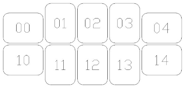
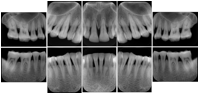
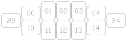
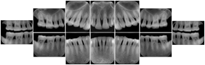
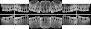
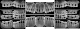
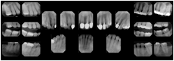
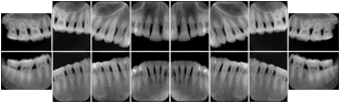
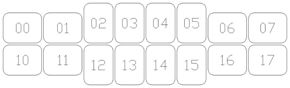
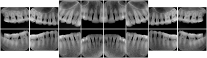
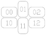
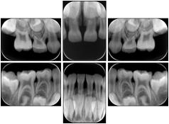
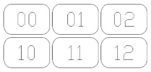
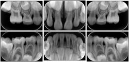
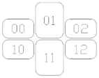
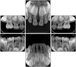
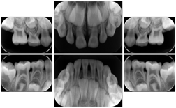
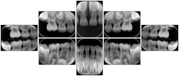
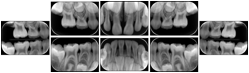
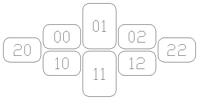
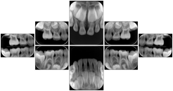
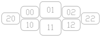
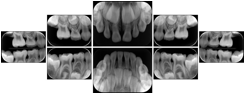
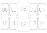
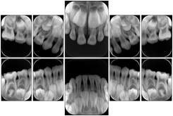
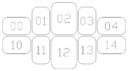
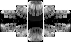
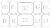
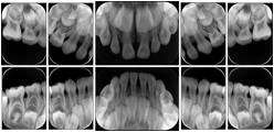
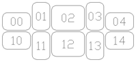
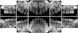
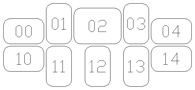
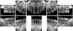
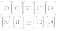
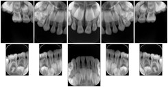
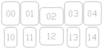
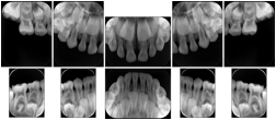
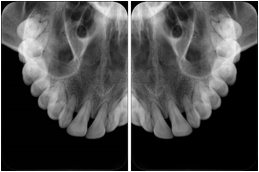
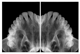
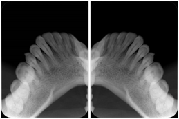
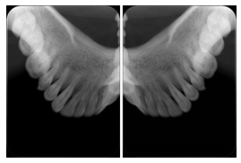
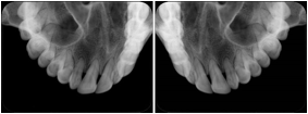
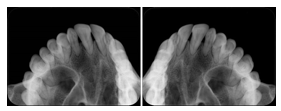
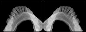
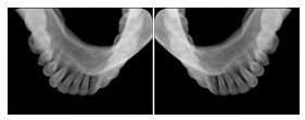
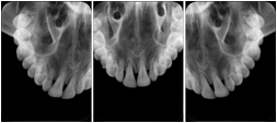
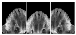
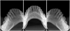
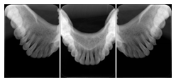
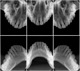
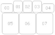
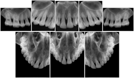
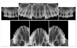
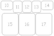
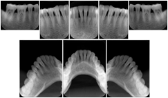
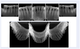
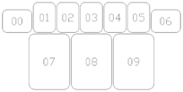
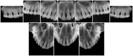
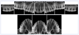
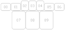
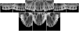
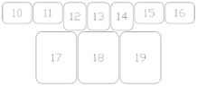
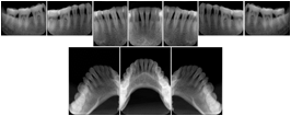
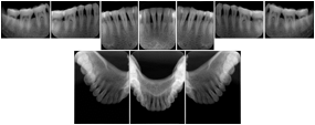
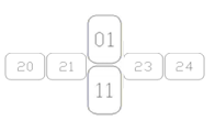
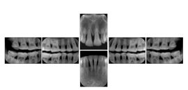
A patient in rural Canada visits a general ophthalmologist and is found to have diabetic macular edema. The general ophthalmologist would like to discuss the case with a retina specialist before performing laser surgery. A fluorescein angiogram is done with multiple retinal images taken in a timed series after an intravenous injection. The images along with a Structured Display are shared via a Health Information Exchange with a retina specialist in Calgary, who opens them using his Ophthalmology EMR software and consults via phone with the general ophthalmologist. Both physicians view the images in the same layout so the retina specialist can provide accurate guidance for treating the patient.
A patient in rural Iowa visits his primary care physician for management of diabetes. Three non-mydriatic (patient's eyes are not dilated) photographs are taken of the back of each eye, and forwarded electronically along with a Structured Display to an ophthalmologist in Iowa City. The ophthalmologist reads the photos in an agreed upon layout so there is no mistake about what portion of which eye is being viewed. The ophthalmologist is able to tell the primary care physician that his patient does not need to come to Iowa City for face to face ophthalmologic care, but that there is a particular view of the left eye that should be photographed again in 6 months.

Figure OO-3. Ophthalmic Retinal Study Structured Display
A patient in rural Minnesota experiences sudden vision loss and goes to a general ophthalmologist, who acquires OCT images and forwards them electronically along with a Structured Display to a retina specialist six travel hours away. The retina specialist is able to view the images in the standard layout that he is comfortable with, and to confirm that the patient has a choroidal neovascular membrane. He determines that is would be worthwhile for the patient to travel for treatment.

Figure OO-4. OCT Retinal Study with Cross Section and Navigation Structured Display

OO.1.3 Cardiology

Cardiac stress testing acquires images in at least two patient states, rest and stress, and typically with several different views of the heart to highlight function of different cardiac anatomic regions. Image review typically involves simultaneous display of the same anatomy at two patient states, or multiple anatomic views at one patient state, or even simultaneous display of multiple anatomic views at multiple states. This applies to all cardiac imaging modalities, including ultrasound, nuclear, and MR. The American College of Cardiology and American Society of Nuclear Medicine have adopted standard display layouts for nuclear cardiology rest-stress studies.

Figure OO-5. Stress Echocardiography Structured Display

Figure OO-6. Stress-Rest Nuclear Cardiography Structured Display

OO.1.4 Radiology

A radiologist on his PACS assembles a screen layout of a stack of CT images of a current lung study, a secondary capture of a 3-D rendering of the CT, and a prior chest radiograph for the patient. He adjusts the window width / window level for the CT images, and zooms and annotates the radiograph to clearly indicate the tumor. He saves a Structured Display object representing that screen layout, including Grayscale Softcopy Presentation State objects for the CT WW/WL and the radiograph zoom and annotation. During the weekly radiology department conference, on an independent (non-PACS) workstation, he accesses the Structured Display object, and the display workstation automatically loads and places the images on the display, and presents them with the recorded WW/WL, zoom settings, and annotations.
A mammographer reviews a screening exam on a mammo workstation. She wishes to discuss the exam with the patient's general practitioner, who does not have a mammo-specific workstation. She saves a structured display, with presentation states for each image that replicate the display rendered by the mammo workstation (scaling, horizontal and vertical alignment, view and laterality annotation, etc.).

Figure OO-7. Mammography Structured Display

PP 3D Ultrasound Volumes (Informative)

PP.1 Purpose of This Annex

The purpose of this annex is to identify the clinical use cases that drove the development of Enhanced US Volume Object Definition for 3D Ultrasound image storage. They represent the clinical needs that must be addressed by interoperable Ultrasound medical devices and compatible workstations exchanging 3D Ultrasound image data. The use cases listed here are reviewed by representatives of the clinical community and are believed to cover most common applications of 3D Ultrasound data sets.

PP.2 3D Ultrasound Clinical Use Cases

PP.2.1 Use Cases

The following use cases consider the situations in which 3D Ultrasound data is produced and used in the clinical setting:

An ultrasound scanner generates a Volume Data set consisting of a set of parallel XY planes whose positions are specified relative to each other and/or a transducer frame-of-reference, with each plane containing one or more frames of data of different ultrasound data types. Ultrasound data types include, but are not limited to reflector intensity, Doppler velocity, Doppler power, Doppler variance, etc.
An ultrasound scanner generates a set of temporally related Volume Data sets, each as described in Case1. Includes a set of volumes that are acquired sequentially, or acquired asynchronously and reassembled into temporal sequence (such as through the "Spatial-Temporal Image Correlation" (STIC) technique).
Any Volume Data set may be operated upon by an application to create one or more Multi-Planar Reconstruction (MPR) views (as in Case7)
Any Volume Data set may be operated upon by an application to create one or more Volume Rendered views (as in Case8)
Make 3D size measurements on a volume in 3D-space
An ultrasound scanner generates 3D image data consisting of one or more 2D frames that may be displayed, including
1. A single 2D frame
2. A temporal loop of 2D frames
3. A loop of 2D frames at different spatial positions and/or orientations positions relative to one another
4. A loop of 2D frames at different spatial positions, orientations, and/or times relative to one another
An ultrasound scanner generates 3D image data consisting of one or more MPR Views that may be displayed as ordinary 2D frames, including
1. An MPR View
2. A temporal loop of MPR Views
3. A loop of MPR Views representing different spatial positions and/or orientations relative to one another
4. A loop of MPR Views representing different spatial positions, orientations, and/or times relative to one another
5. A collection of MPR Views related to one another (example: 3 mutually orthogonal MPR Views around the point of intersection)
An ultrasound scanner generates 3D image data consisting of one or more Volume Rendered Views that may be displayed as ordinary 2D frames, including
1. An Rendered View
2. A temporal loop of Rendered Views
3. A loop of Rendered Views with a varying observer point
4. A temporal loop of Rendered Views with a varying observer point
Note

Images in this group are not normally measurable because each pixel in the 2D representation may be comprised of data from many pixels in depth along the viewing ray and does not correspond to any particular point in 3D-space.
Allow successive display of frames in multi-frame objects in cases 6, 7, and 8.
Make size measurements on 2D frames in cases 6, 7, and 8.
Separation of different data types allows for independent display and/or processing of image data (for example, color suppression to expose tissue boundaries, grayscale suppression for vascular flow trees, elastography, etc.)
Represent ECG and other physiological waveforms synchronized to acquired images.
Two-stage Retrieval: The clinician initially queries for and retrieves all the images in an exam that are directly viewable as sets of frames. Based on the review of these images (potentially on a legacy review application), the clinician may decide to perform advanced analysis of a subset of the exam images. Volume Data sets corresponding to those images are subsequently retrieved and examined.
An ultrasound scanner allows user to specify qualitative patient orientation (e.g., Left, Right, Medial, etc.) along with the image data.
An ultrasound scanner may maintain a patient-relative frame of reference (obtained such as through a gantry device) along with the image data.
Fiducial markers that tag anatomical references in the image data may be specified along with the image data.
Key Images of clinical interest are identified and either the entire image, or one or more frames or a volume segmentation within the image must be tagged for later reference.

PP.2.2 Hierarchy of Use Cases

This section organizes the list of use cases into a hierarchy. Section PP.3 maps items in this hierarchy to specific solutions in the DICOM Standard.

Data
1. 3D Volume Data
  1. Static and Dynamic volume data sets (Cases 1 and 2)
  2. Suitable for applications that create MPR and Render views (Cases 3 and 4)
  3. 3D size measurements (Case 5)
2. 2D representations of 3D volume data (Cases 6, 7, and 8)
  1. Static and Dynamic varieties (Case 9)
  2. 2D size measurements (Case 10)
3. Separation of data types (Case 11)
4. Integrate physiological waveforms with image acquisition (Case 12)
Workflow
1. Permit Two-step review (Case 13)
  1. Review 2D representations first (potentially on legacy viewer)
  2. On-demand operations on 3D volume data set
2. Frame of Reference
  1. Frame-relative
  2. Probe-relative
  3. Patient-relative (Cases 14 and 15)
  4. Anatomical (Fiducials) (Case 16)
3. Identify Key images (Case 17)

PP.3 3D Ultrasound Solutions in DICOM

This section maps the use case hierarchy in Section PP.2.2 to specific solutions in the DICOM Standard. As described in items 1a and 1b, there are two different types of data related to 3D image acquisition: the 3D volume data set itself and 2D images derived from the volume data set. See Figure PP.3-1.

Figure PP.3-1. Types of 3D Ultrasound Source and Derived Images

PP.3.1 3D Volume Data sets

The 3D volume data set is conveyed via the Enhanced US Volume SOP Class, which represents individual 3D Volume Data sets or collections of temporally-related 3D Volume Data sets using the 'enhanced' multi-frame features used by Enhanced Storage SOP Classes for other modalities, including shared and per-frame functional group sequences and multi-frame dimensions. The 3D Volume Data sets represented by the Enhanced Ultrasound IOD (the striped box in Figure PP.3-1) are suitable for Multi-Planar Reconstruction (MPR) and 3D rendering operations. Note that the generation of the Cartesian volume, its relationship to spatially-related 2D frames (whether the volume was created from spatially-related frames, or spatially-related frames extracted from the Cartesian volume), and the algorithms used for MPR or 3D rendering operations are outside the scope of this standard.

Functional Group Macros allow the storage of many parameters describing the acquisition and positioning of the image planes relative to the patient and external frame of references (such as a gantry or probe locating device). These macros may apply to the entire instance (Shared Functional Group) or may vary frame-to-frame (Per-Frame Functional Group).

Multi-frame Dimensions are used to organize the data type, spatial, and temporal variations among frames. Of particular interest is Data Type used as a dimension to relate frames of different data types (like tissue and flow) comprising each plane of an ultrasound image (item 1c in the use case hierarchy). Refer to Section C.8.24.3.3 for the use of Dimensions with the Enhanced US Volume SOP Class.

Sets of temporally-related volumes may have been acquired sequentially or acquired asynchronously and reassembled into a temporal sequence, such as through Spatial-Temporal Image Correlation (STIC). Regardless of how the temporal volume sequence was acquired, frames in the resultant volumes are marked with a temporal position value, such as Temporal Position Time Offset (0020,930D) indicating the temporal position of the resultant volumes independent of the time sequence of the acquisition prior to reassembly into volumes.

PP.3.2 2D Derived Images

The 2D image types represent collections of frames that are related to or derived from the volume data set, namely Render Views (projections), separate Multi-Planar Reconstruction (MPR) views, or sets of spatially-related source frames, either parallel or oblique (the cross-hatched images in Figure PP.3-1). The Ultrasound Image and Ultrasound Multi-frame Image IODs are used to represent these related or derived 2D images. The US Image Module for the Ultrasound Image Storage and Ultrasound Multi-frame Image Storage SOP Classes have defined terms for "3D Rendering" (render or MPR views) and "Spatially Related Frames" in value 4 of the Image Type (0008,0008) attribute to specify that the object contains these views while maintaining backwards compatibility with Ultrasound review applications for frame-by-frame display, which may be displayed sequentially ("fly-through" or temporal) loop display or as a side-by-side ("light-box") display of spatially-related slices. Also, the optional Source Image Sequence (0008,2112) and Derivation Code Sequence (0008,9215) attributes may be included to more succinctly specify the type of image contained in the instance and the 3D Volume Data set from which it was derived.

2D Derived image instances should be linked to the source 3D Volume Data set through established DICOM reference mechanisms. This is necessary to support the "Two-Stage Review" use case. Consider the following examples:

In the case of a 3D Volume Data set created from a set of spatially-related frames within the ultrasound scanner,
- the Enhanced US Volume instance should include
  1. Referenced Image Sequence (0008,1140) to the source Ultrasound Image and/or Multi-frame Image instances
  2. Referenced Image Purpose of Reference Code Sequence (0040,A170) using (121346, DCM, "Acquisition frames corresponding to volume")
- and the Ultrasound Image and/or Multi-frame Image instances should include:
  1. Referenced Image Sequence (0008,1140) to the 3D Volume Data set
  2. Referenced Image Purpose of Reference Code Sequence (0040,A170) using (121347, DCM, "Volume corresponding to spatially-related acquisition frames")
In the case of an Ultrasound Image or Ultrasound Multi-frame Image instance containing one or more of the spatially-related frames derived from a 3D volume data set, the ultrasound image instance should include:
1. Source Image Sequence (0008,2112) referencing the Enhanced US Volume instance
2. Source Image Sequence Purpose of Reference Code Sequence (0040,A170) using (121322, DCM, "Source of Image Processing Operation")
3. Derivation Code Sequence (0008,9215) using (113091, DCM, "Spatially-related frames extracted from the volume")
In the case of separate MPR or 3D rendered views derived from a 3D Volume Data set, the image instance(s) should include:
1. Source Image Sequence (0008,2112) referencing the Enhanced US Volume instance
2. Source Image Sequence Purpose of Reference Code Sequence (0040,A170) using (121322, DCM, "Source of Image Processing Operation")
3. Derivation Code Sequence (0008,9215) using CID 7203 “Image Derivation” code(s) describing the specific derivation operation(s)

PP.3.3 Physiological Waveforms Associated With 3D Volume Data sets

ECG or other physiological waveforms associated with an Enhanced US Volume (item 1d in the use case hierarchy) are to be conveyed via a one or more companion instances of Waveform IODs linked bidirectionally to the Enhanced US Volume instance. Physiological waveforms associated with Ultrasound image acquisition may be represented using any of the Waveform IODs, and are linked with the Enhanced US Volume instance and to other simultaneous waveforms through the Referenced Instance Sequence in the image instance and each waveform instance. The Synchronization module and the Acquisition DateTime attribute (0018,1800) are used to synchronize the waveforms with the image and each other.

PP.3.4 Workflow Considerations

The use case of two-step review (item 2a in the use case hierarchy) is addressed by the use of separate SOP Classes for 2D and 3D data representations. A review may initially be performed on the Ultrasound Image and Ultrasound Multi-frame image instances created during the study. If additional operations on the 3D volume data set are desired, the Enhanced US Volume instance referenced in the Source Image Sequence of the derived object may be individually retrieved and operated upon by an appropriate application.

The 3D volume data set spatially relates individual frames of the image to each other using the Transducer Frame of Reference defined in Section C.8.24.2 in PS3.3 (items 2b in the use case hierarchy). This permits alignment of frames with each other in the common situation where a hand-held ultrasound transducer is used without an external frame of reference. However, the Transducer Frame of Reference may in turn be related to an external Frame of Reference through the Transducer Gantry Position and Transducer Gantry Orientation attributes. This would permit the creation of optional Image Position and Orientation values relative to the Patient when this information is available. In addition to these frames of reference, the spatial registration, fiducials, segmentation, and deformation objects available for other Enhanced objects may also be used with the Enhanced US Volume instances.

The Key Object Selection Document SOP Class may be used to identify specific Enhanced US Volume instances of particular interest (item 2d in the use case hierarchy).

QQ Enhanced US Data Type Blending Examples (Informative)

QQ.1 Enhanced US Volume Use of the Blending and Display Pipeline

This Annex contains a number of examples illustrating Ultrasound's use of the Blending and Display Pipeline. An overview of the examples included is found in Table QQ.1-1.

Table QQ.1-1. Enhanced US Data Type Blending Examples (Informative)

Example	Data Types	Blending RGB Inputs	Mapping	Blending Operation	Blending Weight Inputs
1	TISSUE_INTENSITY	NA	Identity	None	NA
2	TISSUE_INTENSITY	RGB1 = grayscale TISSUE_INTENSITY	Grayscale	Output = RGB1	Weight 1 = 1.0 (constant)
2	TISSUE_INTENSITY	RGB1 = grayscale TISSUE_INTENSITY	Grayscale	Output = RGB1	Weight 2 = 0.0 (constant)
3	TISSUE_INTENSITY	RGB1 = f(TISSUE_INTENSITY)	Colorized	Output = RGB1	Weight 1 = 1.0 (constant)
3	TISSUE_INTENSITY	RGB1 = f(TISSUE_INTENSITY)	Colorized	Output = RGB1	Weight 2 = 0.0 (constant)
4	TISSUE_INTENSITY	RGB1 = grayscale TISSUE_INTENSITY	Grayscale	Output = proportional summation of RGB1 and RGB2	Weight 1 = constant
4	FLOW_VELOCITY	RGB2 = g(FLOW_VELOCITY)	Colorized	Output = proportional summation of RGB1 and RGB2	Weight 2 = constant
5	TISSUE_INTENSITY	RGB1 = grayscale TISSUE_INTENSITY	Grayscale	Threshold based on FLOW_VELOCITY	Weight 1 = 1 - Alpha 2
5	FLOW_VELOCITY	RGB2 = g(FLOW_VELOCITY)	Colorized	Threshold based on FLOW_VELOCITY	Weight 2 = constant
6	TISSUE_INTENSITY	RGB1 = grayscale TISSUE_INTENSITY	Grayscale	Threshold based on FLOW_VELOCITY (MSB) and FLOW_VARIANCE (LSB) with 2-dimensional color mapping	Weight 1 = 1 - Alpha 2
	FLOW_VELOCITY	RGB2 = g(FLOW_VELOCITY, FLOW_ VARIANCE)	Colorized		Weight 2 = Alpha 2
	FLOW_ VARIANCE	RGB2 = g(FLOW_VELOCITY, FLOW_ VARIANCE)	Colorized		Weight 2 = Alpha 2
7	TISSUE_INTENSITY	RGB1 = f(TISSUE_INTENSITY)	Colorized	Combination based on all data value inputs with colorized tissue and colorized 2-dimensional color mapping of flow and variance.	Weight 1 = Alpha 1
	FLOW_VELOCITY	RGB2 = g(FLOW_VELOCITY, FLOW_ VARIANCE)	Colorized		Weight 2 = Alpha 2
	FLOW_ VARIANCE	RGB2 = g(FLOW_VELOCITY, FLOW_ VARIANCE)	Colorized		Weight 2 = Alpha 2

In the examples below, the following attributes are referenced:

Data Type (0018,9808)
Data Path Assignment (0028,1402)
Bits Mapped to Color Lookup Table (0028,1403)
Blending LUT 1 Transfer Function (0028,1405)
Blending LUT 2 Transfer Function (0028,140D)
Blending Weight Constant (0028,1406)
RGB LUT Transfer Function (0028,140F)
Alpha LUT Transfer Function (0028,1410)
Red Palette Color Lookup Table Descriptor (0028,1101)
Red Palette Color Lookup Table Data (0028,1201)
Green Palette Color Lookup Table Descriptor (0028,1102)
Green Palette Color Lookup Table Data (0028,1202)
Blue Palette Color Lookup Table Descriptor (0028,1103)
Blue Palette Color Lookup Table Data (0028,1203)
Alpha Palette Color Lookup Table Descriptor (0028,1104)
Alpha Palette Color Lookup Table Data (0028,1204)

QQ.1.1 Example 1 - Grayscale P-Values Output

Grayscale pass through for 1 data frame using identity Presentation LUT:

Data Type	Data Path Assignment	Usage
TISSUE_INTENSITY	PRIMARY_PVALUES	Grayscale

Figure QQ.1-1. Example 1

QQ.1.2 Example 2 - Grayscale-only Color Output

Grayscale mapping only from 1 data frame:

Weight 1:
- Blending LUT 1 Transfer Function = CONSTANT
- Blending Weight Constant = 1.0
Weight 2:
- Blending LUT 2 Transfer Function = CONSTANT
- Blending Weight Constant = 0.0
Primary Palette Color Lookup Table
- RGB LUT Transfer Function = EQUAL_RGB
- Alpha LUT Transfer Function = not significant with these Blending LUT Transfer Function values
Secondary Palette Color Lookup Table
- <none>

Note

Compared to Example 1, the perceived contrast of the displayed grayscale image will likely be different as a consequence of the use of PCS-Values as opposed to P-Values unless color management software interpreting the PCS-Values attempts to approximate the Grayscale Standard Display Function. This is true regardless of whether a color or grayscale display is used.

Data Type	Data Path Assignment	Usage
TISSUE_INTENSITY	PRIMARY_SINGLE	Mapped to Grayscale

Figure QQ.1-2. Example 2

QQ.1.3 Example 3 - Color Tissue (Pseudo-color) Mapping

Grayscale mapping only from 1 data frame:

Weight 1:
- Blending LUT 1 Transfer Function = CONSTANT
- Blending Weight Constant = 1.0
Weight 2:
- Blending LUT 2 Transfer Function = CONSTANT
- Blending Weight Constant = 0.0
Primary Palette Color Lookup Table
- RGB LUT Transfer Function = TABLE
- Alpha LUT Transfer Function = not significant with these Blending LUT Transfer Function values
- Red, Green, and Blue Palette Color Lookup Table Descriptors and Data included
Secondary Palette Color Lookup Table
- <none>

Data Type	Data Path Assignment	Usage
TISSUE_INTENSITY	PRIMARY_SINGLE	Mapped through Palette Color Lookup Table

Figure QQ.1-3. Example 3

QQ.1.4 Example 4 - Fixed Proportion Additive Grayscale Tissue and Color Flow

Grayscale mapping from primary data frame and color mapping from secondary data frame:

Weight 1:
- Blending LUT 1 Transfer Function = CONSTANT
- Blending Weight Constant = value between 0.0 and 1.0, inclusive
Weight 2:
- Blending LUT 2 Transfer Function = CONSTANT
- Blending Weight Constant = value between 0.0 and 1.0, inclusive
Primary Palette Color Lookup Table
- RGB LUT Transfer Function = EQUAL_RGB
- Alpha LUT Transfer Function = not significant with these Blending LUT Transfer Function values
Secondary Palette Color Lookup Table
- RGB LUT Transfer Function = TABLE
- Alpha LUT Transfer Function = not significant with these Blending LUT Transfer Function values
- Red, Green, and Blue Palette Color Lookup Table Descriptors and Data included

Data Type	Data Path Assignment	Usage
TISSUE_INTENSITY	PRIMARY_SINGLE	Mapped to Grayscale
FLOW_VELOCITY	SECONDARY_SINGLE	Mapped through Palette Color Lookup Table

Figure QQ.1-4. Example 4

QQ.1.5 Example 5 - Threshold Based On Flow_velocity

Each output value is either the grayscale tissue intensity value or the colorized flow velocity value based on the magnitude of the flow velocity sample value:

Weight 1:
- Blending LUT 1 Transfer Function = ALPHA_2
Weight 2:
- Blending LUT 2 Transfer Function = ONE_MINUS
Primary Palette Color Lookup Table
- RGB LUT Transfer Function = EQUAL_RGB
- Alpha LUT Transfer Function = not significant with these Blending LUT Transfer Function values
Secondary Palette Color Lookup Table
- RGB LUT Transfer Function = TABLE
- Alpha LUT Transfer Function = TABLE
- Red, Green, Blue, and Alpha Palette Color Lookup Table Descriptors and Data included
- All Alpha Palette Color Lookup Table Data values (normalized) are either 0.0 or 1.0

Data Type	Data Path Assignment	Usage
TISSUE_INTENSITY	PRIMARY_SINGLE	Mapped to Grayscale
FLOW_VELOCITY	SECONDARY_SINGLE	Mapped through Palette Color Lookup Table

Figure QQ.1-5. Example 5

QQ.1.6 Example 6 - Threshold Based On Flow_velocity and Flow_variance W/2d Color Mapping

Each output value is either the grayscale tissue intensity value or a colorized flow/variance value determined by a 2-dimensional Secondary RGB Palette Color Lookup Table, based on flow/variance values. The colorized flow/variance value comes from a 2-dimensional Secondary RGB Palette Color LUT:

Weight 1:
- Blending LUT 1 Transfer Function = ALPHA_2
Weight 2:
- Blending LUT 2 Transfer Function = ONE_MINUS
Primary Palette Color Lookup Table
- RGB LUT Transfer Function = EQUAL_RGB
- Alpha LUT Transfer Function = not significant with these Blending LUT Transfer Function values
Secondary Palette Color Lookup Table
- RGB LUT Transfer Function = TABLE
- Alpha LUT Transfer Function = TABLE
- Red, Green, Blue, and Alpha Palette Color Lookup Table Descriptors and Data included
- All Alpha Palette Color Lookup Table Data values (normalized) are either 0.0 or 1.0

Data Type	Data Path Assignment	Usage
TISSUE_INTENSITY	PRIMARY_SINGLE	Mapped to Grayscale
FLOW_VELOCITY	SECONDARY_HIGH	MSBs of index to Palette Color LUT
FLOW_VARIANCE	SECONDARY_LOW	LSBs of index to Palette Color LUT

Figure QQ.1-6. Example 6

QQ.1.7 Example 7 - Color Tissue / Velocity / Variance Mapping - Blending Considers Both Data Paths

Each output value is a combination of colorized tissue intensity and a colorized flow/variance value determined by a 2-dimensional Secondary RGB Palette Color Lookup Table using the upper 5 bits of the FLOW_VELOCITY value and upper 3 bits of the FLOW_VARIANCE value to allow the use of 256-value Secondary Palette Color Lookup Tables. The blending proportion is based on values from both data paths. If the sum of the two RGB values exceeds 1.0, the value is clamped to 1.0. The colorized flow/variance value comes from a 2-dimensional Secondary RGB Palette Color LUT:

Weight 1:
- Blending LUT 1 Transfer Function = ALPHA_1
Weight 2:
- Blending LUT 2 Transfer Function = ALPHA_2
Primary Palette Color Lookup Table
- RGB LUT Transfer Function = TABLE
- Alpha LUT Transfer Function = TABLE
- Red, Green, Blue, and Alpha Palette Color Lookup Table Descriptors and Data included
Secondary Palette Color Lookup Table
- RGB LUT Transfer Function = TABLE
- Alpha LUT Transfer Function = TABLE
- Red, Green, Blue, and Alpha Palette Color Lookup Table Descriptors and Data included

Data Type	Data Path Assignment	Bits Mapped To Color Lookup Table	Usage
TISSUE_INTENSITY	PRIMARY_SINGLE	8	Mapped through Palette Color Lookup Table
FLOW_VELOCITY	SECONDARY_HIGH	5	MSBs of index to Palette Color LUT
FLOW_VARIANCE	SECONDARY_LOW	3	LSBs of index to Palette Color LUT

Figure QQ.1-7. Example 7

RR Ophthalmic Refractive Reports Use Cases (Informative)

RR.1 Introduction

Refractive instruments are the most commonly used instruments in eye care. At present many of them have the capability for digital output, but their data is most often addressed by manual input into a paper or electronic record.

Refractive instruments address the power of a lens or of a patient's eye to bend light. In order for a patient to see well light must be focused on the retina in the back of the eye. If the natural optics of a patient's eye do not accomplish this, corrective lenses can bend incident light so that it will be focused on the retina after passing through the optics of the eye. The power of an optical system such as a spectacle lens or the eye is measured by its ability to bend light, and is measured in diopters (D). In practical clinical applications, this is measured to 3 decimal points, in increments of 0.125 D. The power of a lens is measured in at least two major meridians. A spherical lens power occurs when the power is the same in all meridians (0-180 degrees). A cylindrical lens power occurs when there is a difference in lens power across the various meridians. The shape of the anterior surface of the eye largely determines what type of correcting lens is needed. An eye that requires only spherical lens power is usually shaped spherically, more like a ball, while an eye that requires cylindrical lens power is ellipsoid and shaped more like a football.

Lenses can also bend light without changing its focal distance. This type of refraction simply displaces the position of the image laterally. The power of a prism to bend light is measured in prism diopters. In practical clinical applications this is measured to 1 decimal point, in increments of 0.5 prism diopters. Prism power is required in a pair of spectacles most commonly when both eyes are not properly aligned with the object of regard. Clinical prisms are considered to bend all light coming in from the lens either up, down, in toward the nose, or out away from the nose, in order to compensate for ocular misalignment.

Visual acuity is measured in various scales, all of which indicate a patient's vision as a fraction of what a reference standard patient would see at any given distance. For example, if a patient has 20/30 vision it means that he sees from a distance of 20 feet what a reference standard patient would see from a distance of 30 feet. These measurements are determined by presentation of standardized objects or symbols (optotypes) of varying sizes calibrated to reference standard vision (20/20). The smallest discernible optotype defines the patient's visual acuity expressed in a variety of formats (letters, numbers, pictures, tumbling E, Landolt C, etc).

Visual acuity is measured in two categories of viewing distances: distance, and near. Distance visual acuity is measured at 20' or six meters. This distance is roughly equivalent to optical infinity for clinical purposes. The near viewing distance can vary from 30cm to 75 cm depending on a variety of other conditions, but most commonly is measured at 40 cm.

Visual acuity is measured under several common viewing conditions: 1) Uncorrected vision is measured using the autoprojector to project the above mentioned optotypes for viewing, with no lenses in front of the patient's eyes. The line of smallest optotypes of which the patient can see more than half is determined, and that information is uploaded to a computer system. 2) The patient's vision using habitual correction is measured in a similar fashion using whichever vision correction the patient customarily wears. 3) Pinhole vision is measured in a similar fashion, with the patient viewing the optotypes through a pinhole occluder held in front of the eye. Pinhole visual acuity testing reduces retinal blur, providing an approximation of what the patient's vision should be with the best possible refractive correction (spectacles) in place. 4) Best corrected visual acuity is the visual acuity with the best refractive correction in place. 5) Crowding visual acuity measures the presence and amount of disparity in acuity between single optotype and multiple optotype presentations.

A patient's spectacle prescription may or may not represent the same lenses that provided best corrected visual acuity in his refraction. Subjective comfort plays a role in determining the final spectacle prescription.

Autolensometer: an autolensometer is used to measure the refractive power of a patient's spectacles. This is done by the automatic analysis of the effect of the measured lens upon a beam of light passing through it. Output from an autolensometer can be uploaded to a phoropter to provide a baseline for subjective refraction (discussed below), and it can be uploaded to a computerized medical record. Lenses may also be measured to confirm manufacturing accuracy.
Autorefractor: an autorefractor is used to automatically determine, without patient input, what refractive correction should provide best corrected visual acuity. Output from an autorefractor can be uploaded to a phoropter to provide a baseline for subjective refraction (discussed below), and it can be uploaded to a computerized medical record.
Phoropter (or phoroptor):an instrument containing multiple lenses, that is used in the course of an eye exam to determine the individual's subjective response to various lenses (subjective refraction) and the need for glasses or contact lenses.. The patient looks through the phoropter lenses at an eye chart that may be at 20 ft or 6m or at a reading chart that may be at 40 cm. Information from the subjective refraction can be uploaded from an autophoropter to a computer. The best corrected vision that was obtained is displayed in an autoprojector, and that information can also be uploaded to a computer.
Autokeratometer: an autokeratometer is used to measure the curvature, and thus the refractive power, of a patient's cornea. Two measurements are generally taken, one at the steepest and one at the flattest meridian of the cornea. The meridian measured is expressed in degrees, whole integers, in increments of 1 degree. If the measurement is expressed as power, the unit of measurement is diopters, to 3 decimal points, in increments of 0.125D. If the measurement is expressed as radius of curvature, the unit of measurement is millimeters, to 2 decimal points, in increments of 0.01 mm.

RR.2 Reference Tables For Equivalent Visual Acuity Notations

RR.2.1 Background

Visual acuity is defined as the reciprocal of the ratio between the letter size that can just be recognized by a patient, relative to the size just recognized by a standard eye. If the patient requires letters that are twice as large (or twice as close), the visual acuity is said to be 1/2; if the letters need to be 5x larger, visual acuity is 1/5, and so on.

Note that the scales in the tables extend well above the reference standard (1.0, 20/20, the ability to recognize a letter subtending a visual angle 5 min. of arc), since normal acuity is often 1.25 (20/16), 1.6 (20/12.5) or even 2.0 (20/10).

Today, the ETDRS chart and ETDRS protocol, established by the National Eye Institute in the US, are considered to represent the de facto gold standard for visual acuity measurements The International Council Of Ophthalmology, Visual Standard, Aspects and Ranges of Vision Loss (April, 2002) is a good reference document.

The full ETDRS protocol requires a wide chart, in the shape of an inverted triangle, on a light box, and cannot be implemented on the limited screen of a projector (or similar) chart.

For most routine clinical measurements projector charts or traditional charts with a rectangular shape are used; these non-standardized tools are less accurate than ETDRS measurements.

This appendix contains two lookup tables, one for traditional charts and one for ETDRS measurements.

RR.2.2 Notations

Various notations may be used to express visual acuity. Snellen (in 1862) used a fractional notation in which the numerator indicated the actual viewing distance; this notation has long been abandoned for the use of equivalent notations, where the numerator is standardized to a fixed value, regardless of the true viewing distance. In Europe the use of decimal fractions is common (1/2 = 0.5, 1/5 = 0.2); in the US the numerator is standardized at 20 (1/2 = 20/40, 1/5 = 20/100), while in Britain the numerator 6 is common (1/2 = 6/12, 1/5 = 6/30).

The linear scales on the right side of the tables are not meant for clinical records. They are required for statistical manipulations, such as calculation of differences, trends and averages and preferred for graphical presentations. They convert the logarithmic progression of visual acuity values to a linear one, based on Weber-Fechner's law, which states that proportional stimulus increases lead to linear increases in perception.

The logMAR scale is calculated as log (MAR) = log (1/V) = - log (V). LogMAR notation is widely used in scientific publications. Note that it is a scale of vision loss, since higher values indicate poorer vision. The value "0" indicates "no loss", that is visual acuity equal to the reference standard (1.0, 20/20). Normal visual acuity (which is better than 1.0 (20/20) ) is represented by negative logMAR values.

The VAS scale (VAS = Visual Acuity Score) serves the same purpose. Its formula is: 100 - 50 x logMAR or 100 + 50 x log (V). It is more user friendly, since it avoids decimal values and is more intuitive, since higher values indicate better vision. The score is easily calculated on ETDRS charts, where 1 point is credited for each letter read correctly. The VAS scale also forms the basis for the calculation of visual impairment ratings in the AMA Guides to the Evaluation of Permanent Impairment.

RR.2.3 Use of The Lookup Table

Data input: Determine the notation used in the device and the values of the lines presented. No device will display all the values listed in each of the traditional columns. Convert these values to the decimal DICOM storage values shown on the left of the same row. DICOM values are not meant for data display. In the table, they are listed in scientific notation to avoid confusion with display notations.

In the unlikely event that a value must be stored that does not appear in the lookup table, calculate the decimal equivalent and round to the nearest listed storage value.

Data display: If the display notation is the same as the input notation, convert the DICOM storage values back to the original values. If the notation chosen for the display is different from the input notation, choose the value on the same row from a different column. In certain cases this may result in an unfamiliar notation; unfortunately, this is unavoidable, given the differences in size progressions between different charts. If a suffix (see attribute "Visual Acuity Modifiers" (0046,0135) ) is present, that suffix will be displayed as it was recorded.

Suffixes: Suffixes may be used to indicate steps that are smaller than a 1 line difference. On traditional charts, such suffixes have no defined numerical value. Suffixes +1, +2, +3 and -1, -2, -3 may be encountered. These suffixes do not correspond to a defined number of rows in the table.

RR.2.4 Traditional Charts

The Traditional charts used in clinical practice are not standardized; they have an irregular progression of letter sizes and a variable number of characters per line. Measurement accuracy may further suffer from hidden errors that cannot be captured by any recording device, such as an inconsistent, non-standardized protocol, inaccurate viewing distance, inaccurate projector adjustment and contrast loss from room illumination. Therefore, the difference between two routine clinical measurements should not be considered significant, unless it exceeds 5 rows in the table (1 line on an ETDRS chart).

Table RR-1 contains many blank lines to make the vertical scale consistent with that used in Table RR-2. Notations within the same gray band are interchangeable for routine clinical use, since their differences are small compared to the clinical variability, which is typically in the order of 5 rows (1 ETDRS line).

Table RR-1. Reference Table for Use with Traditional Charts

DICOM				Scales for statistics and graphical displays
Decimal Visual Acuity	Traditional scales			Linear Scales
	Decimal	US	6 m	LogMAR	VAS
2.00 E+00	2.0	20/10	6/3	-0.30	115
1.91 E+00				-0.28	114
1.82 E+00				-0.26	113
1.74 E+00				-0.24	112
1.66 E+00				-0.22	111
1.60 E+00	1.6	20/12.5	6/3.8	-0.20	110
1.50 E+00	1.5	20/13	6/4	-0.18	109
1.45 E+00				-0.16	108
1.38 E+00				-0.14	107
1.30 E+00	1.3	20/15	6/4.5	-0.12	106
1.25 E+00	1.25	20/16	6/4.8	-0.10	105
1.20 E+00	1.2	20/17	6/5	-0.08	104
1.15 E+00				-0.06	103
1.10 E+00	1.1	20/18	6/5.5	-0.04	102
1.05 E+00				-0.02	101
1.00 E+00	1.0	20/20	6/6	0	100
9.55 E-01				0.02	99
9.00 E-01	0.9	20/22	6/66	0.04	98
8.70 E-01				0.06	97
8.30 E-01				0.08	96
8.00 E-01	0.8	20/25	6/7.5	0.10	95
7.50 E-01	0.75	20/26	6/8	0.12	94
7.20 E-01				0.14	93
7.00 E-01	0.7	20/28	6/8.7	0.16	92
6.60 E-01	0.66	20/30	6/9	0.18	91
6.30 E-01	0.63	20/32	6/9.5	0.20	90
6.00 E-01	0.6	20/33	6/10	0.22	89
5.75 E-01				0.24	88
5.50 E-01				0.26	87
5.25 E-01				0.28	86
5.00 E-01	0.5	20/40	6/12	0.30	85
4.80 E-01				0.32	84
4.57 E-01				0.34	83
4.37 E-01				0.36	82
4.17 E-01				0.38	81
4.00 E-01	0.4	20/50	6/15	0.40	80
3.80 E-01				0.42	79
3.60 E-01				0.44	78
3.50 E-01				0.46	77
3.33 E-01	0.33	20/60	6/18	0.48	76
3.20 E-01	0.32	20/63	6/19	0.50	75
3.00 E-01	0.3	20/66	6/20	0.52	74
2.90 E-01	0.28	20/70	6/21	0.54	73
2.75 E-01				0.56	72
2.63 E-01				0.58	71
2.50 E-01	0.25	20/80	6/24	0.60	70
2.40 E-01				0.62	69
2.30 E-01				0.64	68
2.20 E-01				0.66	67
2.10 E-01				0.68	66
2.00 E-01	0.2	20/100	6/30	0.70	65
1.90 E-01				0.72	64
1.82 E-01				0.74	63
1.74 E-01				0.76	62
1.66 E-01	0.17	20/120	6/36	0.78	61
1.60 E-01	0.16	20/125	6/38	0.80	60
1.50 E-01	0.15	20/130	6/40	0.82	59
1.45 E-01				0.84	58
1.38 E-01				0.86	57
1.30 E-01	0.13	20/150	6/45	0.88	56
1.25 E-01	0.125	20/160	6/48	0.90	55
1.20 E-01	0.12	20/170	6/50	0.92	54
1.15 E-01				0.94	53
1.10 E-01				0.96	52
1.05 E-01				0.98	51
1.00 E-01	0.1	20/200	6/60	1.00	50
9.55 E-02				1.02	49
9.00 E-02				1.04	48
8.70 E-02				1.06	47
8.30 E-02	0.083	20/240	6/72	1.08	46
8.00 E-02	0.08	20/250	6/75	1.10	45
7.50 E-02				1.12	44
7.20 E-02				1.14	43
7.00 E-02				1.16	42
6.60 E-02	0.065	20/300	6/90	1.18	41
6.30 E-02	0.063	20/320	6/95	1.20	40
6.00 E-02	0.06	20/330	6/100	1.22	39
5.75 E-02				1.24	38
5.50 E-02				1.26	37
5.25 E-02				1.28	36
5.00 E-02	0.05	20/400	6/120	1.30	35
4.80 E-02				1.32	34
4.60 E-02				1.34	33
4.40 E-02				1.36	32
4.20 E-02				1.38	31
4.00 E-02	0.04	20/500	6/150	1.40	30
3.80 E-02				1.42	29
3.60 E-02				1.44	28
3.50 E-02				1.46	27
3.33 E-02				1.48	26
3.20 E-02	0.032	20/630	6/190	1.50	25
3.02 E-02	0.03	20/650	6/200	1.52	24
2.90 E-02				1.54	23
2.75 E-02				1.56	22
2.63 E-02				1.58	21
2.50 E-02	0.025	20/800	6/240	1.60	20
2.40 E-02				1.62	19
2.30 E-02				1.64	18
2.20 E-02				1.66	17
2.10 E-02				1.68	16
2.00 E-02	0.02	20/1000	6/300	1.70	15
1.90 E-02				1.72	14
1.82 E-02				1.74	13
1.74 E-02				1.76	12
1.66 E-02				1.78	11
1.60 E-02	0.016	20/1250	6/380	1.80	10
1.50 E-02	0.015	20/1300	6/400	1.82	9
1.45 E-02				1.84	8
1.38 E-02				1.86	7
1.30 E-02				1.88	6
1.25 E-02	0.0125	20/1600	6/480	1.90	5
1.20 E-02				1.92	4
1.15 E-02				1.94	3
1.10 E-02				1.96	2
1.05 E-02				1.98	1
1.00 E-02	0.01	20/2000	6/600	2.00	0

RR.2.5 ETDRS Charts

ETDRS charts feature Sloan letters with proportional spacing, 5 letters on each line, and a logarithmic progression of letter sizes with consistent increments of approximately 25% per line (10 lines equal a factor 10x). The ETDRS protocol specifies letter-by-letter scoring, viewing distance, illumination, use of different charts for right and left eye and other presentation parameters.

The full ETDRS protocol requires a wide chart on a light box, and cannot be implemented on the limited screen of a projector (or similar) chart. The logarithmic progression, however, can be implemented on any device. This progression was first proposed by John Green in 1868 and follows the standard "Preferred Numbers, ISO standard 3 (1973) " series and the rounding preferences.

Use of ETDRS charts allows use of letter-by-letter scoring, which is more accurate than the line-by-line scoring used on traditional charts. Each row in the table is equivalent to 1 letter on an ETDRS chart (50 letters for a factor 10x). These steps are smaller than the just discernible difference; steps this small only become significant in statistical studies where a large number of measurements is averaged.

The smaller steps for letter by letter scoring may be expressed in two ways; either by using suffixes to a familiar (sometimes slightly rounded) set of values or by using calculated values. For clinical use suffixes have the advantage of using only familiar acuity notations and reverting to the nearest clinical notation when the suffix is omitted. Calculated values look less familiar; but are sometimes used in statistical studies. Note that suffixes used in the context of an ETDRS chart have a defined value and affect the DICOM storage value, whereas suffixes used in the context of traditional charts do not.

Table RR-2. Reference Table for Use with ETDRS Charts or Equivalent

DICOM	Notations for Research Use with ETDRS Charts or Equivalent						Scales for statistics and graphical displays
Decimal Visual Acuity	Use with suffixes			Calculated values			Linear Scales
	Decimal	US	6 m	Decimal	US	6 m	LogMAR	VAS
2.00 E+00	2.0	20/10	6/3	2.00	20/10	6/3.0	-0.30	115
1.91 E+00	-	-	-	1.91	20/10.5	6/3.2	-0.28	114
1.82 E+00	- -	- -	- -	1.82	20/11	6/3.3	-0.26	113
1.74 E+00	+ +	+ +	+ +	1.74	20/11.5	6/3.5	-0.24	112
1.66 E+00	+	+	+	1.66	20/12	6/3.6	-0.22	111
1.60 E+00	1.6	20/12.5	6/3.8	1.58	20/12.5	6/3.8	-0.20	110
1.50 E+00	-	-	-	1.51	20/13	6/4.0	-0.18	109
1.45 E+00	- -	- -	- -	1.45	20/14	6/4.2	-0.16	108
1.38 E+00	+ +	+ +	+ +	1.38	20/14.5	6/4.4	-0.14	107
1.30 E+00	+	+	+	1.32	20/15	6/4.6	-0.12	106
1.25 E+00	1.25	20/16	6/4.8	1.26	20/16	6/4.8	-0.10	105
1.20 E+00	-	-	-	1.20	20/17	6/5.0	-0.08	104
1.15 E+00	- -	- -	- -	1.15	20/17.5	6/5.2	-0.06	103
1.10 E+00	+ +	+ +	+ +	1.10	20/18	6/5.5	-0.04	102
1.05 E+00	+	+	+	1.05	20/19	6/5.8	-0.02	101
1.00 E+00	1.0	20/20	6/6	1.00	20/20	6/6.0	0	100
9.55 E-01	-	-	-	0.95	20/21	6/6.3	0.02	99
9.00 E-01	- -	- -	- -	0.91	20/22	6/6.6	0.04	98
8.70 E-01	+ +	+ +	+ +	0.87	20/23	6/6.9	0.06	97
8.30 E-01	+	+	+	0.83	20/24	6/7.2	0.08	96
8.00 E-01	0.8	20/25	6/7.5	0.79	20/25	6/7.5	0.10	95
7.50 E-01	-	-	-	0.76	20/26	6/7.9	0.12	94
7.20 E-01	- -	- -	- -	0.72	20/28	6/8.3	0.14	93
7.00 E-01	+ +	+ +	+ +	0.69	20/29	6/8.7	0.16	92
6.60 E-01	+	+	+	0.66	20/30	6/9.1	0.18	91
6.30 E-01	0.63	20/32	6/9.5	0.63	20/32	6/9.5	0.20	90
6.00 E-01	-	-	-	0.60	20/33	6/10.0	0.22	89
5.75 E-01	- -	- -	- -	0.58	20/35	6/10.5	0.24	88
5.50 E-01	+ +	+ +	+ +	0.55	20/36	6/11.0	0.26	87
5.25 E-01	+	+	+	0.52	20/38	6/11.5	0.28	86
5.00 E-01	0.5	20/40	6/12	0.50	20/40	6/12.0	0.30	85
4.80 E-01	-	-	-	0.48	20/42	6/12.5	0.32	84
4.57 E-01	- -	- -	- -	0.46	20/44	6/13.2	0.34	83
4.37 E-01	+ +	+ +	+ +	0.24	20/46	6/13.8	0.36	82
4.17 E-01	+	+	+	0.42	20/48	6/14.5	0.38	81
4.00 E-01	0.4	20/50	6/15	0.40	20/50	6/15.1	0.40	80
3.80 E-01	-	-	-	0.38	20/52	6/15.8	0.42	79
3.60 E-01	- -	- -	- -	0.36	20/55	6/16.6	0.44	78
3.50 E-01	+ +	+ +	+ +	0.35	20/58	6/17.4	0.46	77
3.33 E-01	+	+	+	0.33	20/60	6/18.2	0.48	76
3.20 E-01	0.32	20/63	6/19	0.32	20/63	6/19.1	0.50	75
3.00 E-01	-	-	-	0.30	20/66	6/20.	0.52	74
2.90 E-01	- -	- -	- -	0.29	20/69	6/21	0.54	73
2.75 E-01	+ +	+ +	+ +	0.28	20/72	6/22	0.56	72
2.63 E-01	+	+	+	0.26	20/76	6/23	0.58	71
2.50 E-01	0.25	20/80	6/24	0.25	20/79	6/24	0.60	70
2.40 E-01	-	-	-	0.24	20/83	6/25	0.62	69
2.30 E-01	- -	- -	- -	0.23	20/87	6/26	0.64	68
2.20 E-01	+ +	+ +	+ +	0.22	20/91	6/28	0.66	67
2.10 E-01	+	+	+	0.21	20/95	6/29	0.68	66
2.00 E-01	0.2	20/100	6/30	0.20	20/100	6/30	0.70	65
1.90 E-01	-	-	-	0.191	20/105	6/32	0.72	64
1.82 E-01	- -	- -	- -	0.182	20/110	6/33	0.74	63
1.74 E-01	+ +	+ +	+ +	0.174	20/115	6/35	0.76	62
1.66 E-01	+	+	+	0.166	20/120	6/36	0.78	61
1.60 E-01	0.16	20/125	6/38	0.158	20/126	6/38	0.80	60
1.50 E-01	-	-	-	0.151	20/132	6/40	0.82	59
1.45 E-01	- -	- -	- -	0.145	20/138	6/42	0.84	58
1.38 E-01	+ +	+ +	+ +	0.138	20/145	6/44	0.86	57
1.30 E-01	+	+	+	0.132	20/151	6/46	0.88	56
1.25 E-01	0.125	20/160	6/48	0.126	20/158	6/48	0.90	55
1.20 E-01	-	-	-	0.120	20/166	6/50	0.92	54
1.15 E-01	- -	- -	- -	0.115	20/174	6/52	0.94	53
1.10 E-01	+ +	+ +	+ +	0.110	20/182	6/55	0.96	52
1.05 E-01	+	+	+	0.105	20/191	6/58	0.98	51
1.00 E-01	0.1	20/200	6/60	0.100	20/200	6/60	1.00	50
9.55 E-02	-	-	-	0.095	20/210	6/63	1.02	49
9.00 E-02	- -	- -	- -	0.091	20/220	6/66	1.04	48
8.70 E-02	+ +	+ +	+ +	0.087	20/230	6/69	1.06	47
8.30 E-02	+	+	+	0.083	20/240	6/72	1.08	46
8.00 E-02	0.08	20/250	6/75	0.079	20/250	6/76	1.10	45
7.50 E-02	-	-	-	0.076	20/260	6/79	1.12	44
7.20 E-02	- -	- -	- -	0.072	20/280	6/83	1.14	43
7.00 E-02	+ +	+ +	+ +	0.069	20/290	6/87	1.16	42
6.60 E-02	+	+	+	0.066	20/300	6/91	1.18	41
6.30 E-02	0.063	20/320	6/95	0.063	20/315	6/95	1.20	40
6.00 E-02	-	-	-	0.060	20/330	6/100	1.22	39
5.75 E-02	- -	- -	- -	0.058	20/350	6/105	1.24	38
5.50 E-02	+ +	+ +	+ +	0.055	20/360	6/110	1.26	37
5.25 E-02	+	+	+	0.052	20/380	6/115	1.28	36
5.00 E-02	0.05	20/400	6/120	0.050	20/400	6/120	1.30	35
4.80 E-02	-	-	-	0.048	20/420	6/126	1.32	34
4.60 E-02	- -	- -	- -	0.046	20/440	6/132	1.34	33
4.40 E-02	+ +	+ +	+ +	0.044	20/460	6/138	1.36	32
4.20 E-02	+	+	+	0.042	20/480	6/145	1.38	31
4.00 E-02	0.04	20/500	6/150	0.040	20/500	6/151	1.40	30
3.80 E-02	-	-	-	0.038	20/520	6/158	1.42	29
3.60 E-02	- -	- -	- -	0.036	20/550	6/166	1.44	28
3.50 E-02	+ +	+ +	+ +	0.035	20/575	6/174	1.46	27
3.33 E-02	+	+	+	0.033	20/600	6/182	1.48	26
3.20 E-02	0.032	20/630	6/190	0.032	20/630	6/191	1.50	25
3.02 E-02	-	-	-	0.030	20/660	6/200	1.52	24
2.90 E-02	- -	- -	- -	0.029	20/690	6/210	1.54	23
2.75 E-02	+ +	+ +	+ +	0.028	20/720	6/220	1.56	22
2.63 E-02	+	+	+	0.026	20/760	6/230	1.58	21
2.50 E-02	0.025	20/800	6/240	0.025	20/800	6/240	1.60	20
2.40 E-02	-	-	-	0.024	20/830	6/250	1.62	19
2.30 E-02	- -	- -	- -	0.023	20/870	6/260	1.64	18
2.20 E-02	+ +	+ +	+ +	0.022	20/910	6/280	1.66	17
2.10 E-02	+	+	+	0.021	20/950	6/290	1.68	16
2.00 E-02	0.020	20/1000	6/300	0.0200	20/1000	6/300	1.70	15
1.90 E-02	-	-	-	0.0191	20/1050	6/315	1.72	14
1.82 E-02	- -	- -	- -	0.0182	20/1100	6/330	1.74	13
1.74 E-02	+ +	+ +	+ +	0.0174	20/1150	6/350	1.76	12
1.66 E-02	+	+	+	0.0166	20/1200	6/363	1.78	11
1.60 E-02	0.016	20/1250	6/380	0.0158	20/1250	6/380	1.80	10
1.50 E-02	-	-	-	0.0151	20/1300	6/400	1.82	9
1.45 E-02	- -	- -	- -	0.0145	20/1380	6/420	1.84	8
1.38 E-02	+ +	+ +	+ +	0.0138	20/1450	6/440	1.86	7
1.30 E-02	+	+	+	0.0132	20/1500	6/460	1.88	6
1.25 E-02	0.0125	20/1600	6/480	0.0126	20/1600	6/480	1.90	5
1.20 E-02	-	-	-	0.0120	20/1660	6/500	1.92	4
1.15 E-02	- -	- -	- -	0.0115	20/1740	6/520	1.94	3
1.10 E-02	+ +	+ +	+ +	0.0110	20/1820	6/550	1.96	2
1.05 E-02	+	+	+	0.0105	20/1910	6/575	1.98	1
1.00 E-02	0.010	20/2000	6/600	0.0100	20/2000	6/600	2.00	0

SS Colon CAD (Informative)

SS.1 Colon CAD SR Content Tree Structure

The templates for the Colon CAD SR IOD are defined in Colon CAD SR IOD Templates in PS3.16 . All relationships defined in the Colon CAD SR IOD templates are by-value. Content items referenced from another SR object instance, such as a prior Colon CAD SR, are inserted by-value in the new SR object instance, with appropriate original source observation context. It is necessary to update Rendering Intent, and referenced content item identifiers for by-reference relationships, within content items paraphrased from another source.

Figure SS.1-1. Top Levels of Colon CAD SR Content Tree

The Document Root, Image Set Properties, CAD Processing and Findings Summary, and Summaries of Detections and Analyses sub-trees together form the content tree of the Colon CAD SR IOD. See Annex E for additional explanation of the Summaries of Detections and Analyses sub-trees.

The identification of a polyp within an image set is considered to be a Detection. The temporal correlation of a polyp in two image sets taken at different times is considered Analysis. This distinction is used in determining whether to place algorithm identification information in the Summary of Detections or Summary of Analyses sub-trees.

Once a Single Image Finding or Composite Feature has been instantiated, it may be referenced by any number of Composite Features higher in the CAD Processing and Findings Summary sub-tree.

SS.2 Colon CAD SR Observation Context Encoding

Any content item in the Content tree that has been inserted (i.e., duplicated) from another SR object instance has a HAS OBS CONTEXT relationship to one or more content items that describe the context of the SR object instance from which it originated. This mechanism may be used to combine reports (e.g., Colon CAD SR 1, Colon CAD SR 2, Human).

The CAD Processing and Findings Summary section of the SR Document Content tree of a Colon CAD SR IOD may contain a mixture of current and prior single image findings and composite features. The content items from current and prior contexts are target content items that have a by-value INFERRED FROM relationship to a Composite Feature content item. Content items that come from a context other than the Initial Observation Context have a HAS OBS CONTEXT relationship to target content items that describe the context of the source document.

In Figure SS.2-1, Composite Feature and Single Image Finding are current, and Single Image Finding (from Prior) is duplicated from a prior document.

Figure SS.2-1. Example of Use of Observation Context

SS.3 Colon CAD SR Examples

The following is a simple and non-comprehensive illustration of an encoding of the Colon CAD SR IOD for colon computer aided detection results. For brevity, some mandatory content items are not included.

SS.3.1 Example 1: Colon Polyp Detection With No Findings

A colon CAD device processes a typical screening colon case, i.e., there are several hundred images and no polyp findings. Colon CAD runs polyp detection successfully and finds nothing.

The colon radiograph resembles:

Figure SS.3-1. Colon Radiograph as Described in Example 1

The content tree structure would resemble:

Node	Code Meaning of Concept Name	Code Meaning or Example Value	TID
1	Colon CAD Report		TID 4120
1.1	Language of Content Item and Descendants	English	TID 1204
1.2	Image Set Properties		TID 4122
1.2.1	Frame of Reference UID	1.2.840.114191.123	TID 4122
1.2.2	Study Instance UID	1.2.840.114191.456	TID 4122
1.2.3	Study Date	20060924	TID 4122
1.2.4	Study Time	090807	TID 4122
1.2.5	Modality	CT	TID 4122
1.2.6	Horizontal Pixel Spacing	0.80 mm	TID 4122
1.2.7	Vertical Pixel Spacing	0.80 mm	TID 4122
1.2.8	Slice Thickness	2.5 mm	TID 4122
1.2.9	Spacing between slices	1.5 mm	TID 4122
1.2.10	Recumbent Patient Position with respect to gravity	Prone	TID 4122
1.3	CAD Processing and Findings Summary	All algorithms succeeded; without findings	TID 4121
1.4	Summary of Detections	Succeeded	TID 4120
1.4.1	Successful Detections		TID 4015
1.4.1.1	Detection Performed	Nodule	TID 4017
1.4.1.1.1	Algorithm Name	"Colon Polyp Detector"	TID 4019
1.4.1.1.2	Algorithm Version	"V1.3"	TID 4019
1.4.1.1.3	Series Instance UID	1.2.840.114191.789	TID 4017
1.5	Summary of Analyses	Not Attempted	TID 4120

SS.3.2 Example 2: Colon Polyp Detection With Findings

A colon CAD device processes a screening colon case with several hundred images, and a colon polyp detected. The colon radiograph resembles:

Figure SS.3-2. Colon radiograph as Described in Example 2

Figure SS.3-3. Content Tree Root of Example 2 Content Tree

The content tree structure would resemble:

Node	Code Meaning of Concept Name	Code Meaning or Example Value	TID
1	Colon CAD Report		TID 4120
1.1	Language of Content Item and Descendants	English	TID 1204
1.2	Image Set Properties		TID 4122
1.3	CAD Processing and Findings Summary	All algorithms succeeded; with findings	TID 4121
1.4	Summary of Detections	Succeeded	TID 4120
1.5	Summary of Analyses	Not Attempted	TID 4120

Node	Code Meaning of Concept Name	Code Meaning or Example Value	TID
1.2	Image Set Properties		TID 4122
1.2.1	Frame of Reference UID	1.2.840.114191.1122	TID 4122
1.2.2	Study Instance UID	1.2.840.114191.3344	TID 4122
1.2.3	Study Date	20070924	TID 4122
1.2.4	Study Time	090807	TID 4122
1.2.5	Modality	CT	TID 4122
1.2.6	Horizontal Pixel Spacing	0.80 mm	TID 4122
1.2.7	Vertical Pixel Spacing	0.80 mm	TID 4122
1.2.8	Slice Thickness	2.5 mm	TID 4122
1.2.9	Spacing between slices	1.5 mm	TID 4122
1.2.10	Recumbent Patient Position with respect to gravity	Prone	TID 4122

Figure SS.3-4. CAD Processing and Findings Summary Portion of Example 2 Content Tree

Node	Code Meaning of Concept Name	Code Meaning or Example Value	TID
1.3	CAD Processing and Findings Summary	All algorithms succeeded; with findings	TID 4121
1.3.1	Composite Feature	Polyp	TID 4125
1.3.1.1	Rendering Intent	Presentation Required:…	TID 4125
1.3.1.2	Algorithm Name	"Colon Polyp Detector"	TID 4019
1.3.1.3	Algorithm Version	"V1.3"	TID 4019
1.3.1.4	Composite Type	Target content items are related spatially	TID 4126
1.3.1.5	Scope of Feature	Feature detected on multiple images	TID 4126
1.3.1.6	Center	SCOORD3D POINT	TID 4129
1.3.1.7	Outline	SCOORD3D ELLIPSOID	TID 4129
1.3.1.8	Associated Morphology	Pedunculated	TID 4128
1.3.1.9	Diameter	20 mm	TID 1406
1.3.1.9.1	Path	SCOORD3D POLYLINE	TID 1406

Figure SS.3-5. Summary of Detections Portion of Example 2 Content Tree

Node	Code Meaning of Concept Name	Code Meaning or Example Value	TID
1.4	Summary of Detections	Succeeded	TID 4120
1.4.1	Successful Detections		TID 4015
1.4.1.1	Detection Performed	Polyp	TID 4017
1.4.1.1.1	Algorithm Name	"Colon Polyp Detector"	TID 4019
1.4.1.1.2	Algorithm Version	"V1.3"	TID 4019
1.4.1.1.3	Series Instance UID	1.2.840.114191.111222	TID 4017

Node	Code Meaning of Concept Name	Code Meaning or Example Value	TID
1.5	Summary of Analyses	Not Attempted	TID 4120

SS.3.3 Example 3: Colon Polyp Detection, Temporal Differencing With Findings

The patient in Example 2 returns for another colon radiograph. A more comprehensive colon CAD device processes the current colon radiograph, and analyses are performed that determine some temporally related content items for Composite Features. Portions of the prior colon CAD report (Example 2) are incorporated into this report. In the current colon radiograph the colon polyp has increased in size.

Figure SS.3-7. Colon radiographs as Described in Example 3

Node	Code Meaning of Concept Name	Code Meaning or Example Value	TID
1	Colon CAD Report		TID 4120
1.1	Language of Content Item and Descendants	English	TID 1204
1.2	Image Set Properties		TID 4122
1.2.1	Frame of Reference UID	1.2.840.114191.5577	TID 4122
1.2.2	Study Instance UID	1.2.840.114191.7788	TID 4122
1.2.3	Study Date	20080924	TID 4122
1.2.4	Study Time	101827	TID 4122
1.2.5	Modality	CT	TID 4122
1.2.6	Horizontal Pixel Spacing	0.80 mm	TID 4122
1.2.7	Vertical Pixel Spacing	0.80 mm	TID 4122
1.2.8	Slice Thickness	2.5 mm	TID 4122
1.2.9	Spacing between slices	1.5 mm	TID 4122
1.2.10	Recumbent Patient Position with respect to gravity	Prone	TID 4122
1.3	Image Set Properties		TID 4122
1.3.1	Frame of Reference UID	1.2.840.114191.1122	TID 4122
1.3.2	Study Instance UID	1.2.840.114191.3344	TID 4122
1.3.3	Study Date	20070924	TID 4122
1.3.4	Study Time	090807	TID 4122
1.3.5	Modality	CT	TID 4122
1.3.6	Horizontal Pixel Spacing	0.80 mm	TID 4122
1.3.7	Vertical Pixel Spacing	0.80 mm	TID 4122
1.3.8	Slice Thickness	2.5 mm	TID 4122
1.3.9	Spacing between slices	1.5 mm	TID 4122
1.3.10	Recumbent Patient Position with respect to gravity	Prone	TID 4122

Node	Code Meaning of Concept Name	Code Meaning or Example Value	TID
1.4	CAD Processing and Findings Summary	All algorithms succeeded; with findings	TID 4121
1.4.1	Composite Feature	Polyp	TID 4125
1.4.1.1	Rendering Intent	Presentation Required: …	TID 4125
1.4.1.2	Algorithm Name	"Polyp Change"	TID 4019
1.4.1.3	Algorithm Version	"V2.3"	TID 4019
1.4.1.4	Composite Type	Target content items are related temporally	TID 4126
1.4.1.5	Scope of Feature	Feature detected on multiple images	TID 4126
1.4.1.6	Certainty of Feature	85%	TID 4126
1.4.1.7	Associated Morphology	Pedunculated	TID 4128
1.4.1.8	Difference in size	2 mm	TID 4126
1.4.1.8.1		Reference to Node 1.4.1.9.10	TID 4126
1.4.1.8.2		Reference to Node 1.4.1.10.10	TID 4126
1.4.1.9	Composite Feature	Polyp	TID 4125
1.4.1.9.1	Rendering Intent	Presentation Required: …	TID 4125
1.4.1.9.2	Tracking Identifier	"Watchlist #1"	TID 4108
1.4.1.9.3	Algorithm Name	"Colon Polyp Detector"	TID 4019
1.4.1.9.4	Algorithm Version	"V1.3"	TID 4019
1.4.1.9.5	Composite Type	Target content items are related spatially	TID 4126
1.4.1.9.6	Scope of Feature	Feature detected on multiple images	TID 4126
1.4.1.9.7	Center	SCOORD3D POINT	TID 4129
1.4.1.9.8	Outline	SCOORD3D ELLIPSE	TID 4129
1.4.1.9.9	Associated Morphology	Pedunculated	TID 4128
1.4.1.9.10	Diameter	4 mm	TID 1406
1.4.1.9.10.1	Path	SCOORD3D POLYLINE	TID 1406
1.4.1.10	Composite Feature	Polyp	TID 4125
1.4.1.10.1	Rendering Intent	Presentation Required: …	TID 4125
1.4.1.10.2	[Observation Context content items]		TID 4022
1.4.1.10.3	Algorithm Name	"Colon Polyp Detector"	TID 4019
1.4.1.10.4	Algorithm Version	"V1.3"	TID 4019
1.4.1.10.5	Composite Type	Target content items are related spatially	TID 4126
1.4.1.10.6	Scope of Feature	Feature detected on multiple images	TID 4126
1.4.1.10.7	Center	SCOORD3D POINT	TID 4129
1.4.1.10.8	Outline	SCOORD3D ELLIPSE	TID 4129
1.4.1.10.9	Associated Morphology	Pedunculated	TID 4128
1.4.1.10.10	Diameter	2 mm	TID 1406
1.4.1.10.10.1	Path	SCOORD3D POLYLINE	TID 1406
1.5	Summary of Detections	Succeeded	TID 4120
1.5.1	Successful Detections		TID 4015
1.5.1.1	Detection Performed	Polyp	TID 4017
1.5.1.1.1	Algorithm Name	"Colon Polyp Detector"	TID 4019
1.5.1.1.2	Algorithm Version	"V1.3"	TID 4019
1.5.1.1.3	Series Instance UID	1.2.840.114191.555666	TID 4017
1.6	Summary of Analyses	Succeeded	TID 4120
1.6.1	Successful Analyses		TID 4016
1.6.1.1	Analysis Performed	"Temporal correlation"	TID 4018
1.6.1.1.1	Algorithm Name	"Polyp Change"	TID 4019
1.6.1.1.2	Algorithm Version	"V2.3"	TID 4019
1.6.1.1.3	Series Instance UID	1.2.840.114191.111222	TID 4018
1.6.1.1.4	Series Instance UID	1.2.840.114191.555666	TID 4018

TT Stress Testing Report Template (Informative)

The Stress Testing Report is based on TID 3300 “Stress Testing Report”. The first part of the report contains sections (containers) describing the patient characteristics (height, weight, etc.), medical history, and presentation at the time of the exam.

The next part describes the technical aspects of the exam. It includes zero or more findings containers, each corresponding to a phase of the stress testing procedure. Within each container may be one or more sub-containers, each associated with a single measurement set. A measurement set consists of measurements at a single point in time. There are measurement sets defined for both stress monitoring and for imaging.

The final part of the report includes a summary of significant findings or measurements, and any conclusions or recommendations

The resulting hierarchical structure is depicted in Figure TT-1.

Figure TT-1. Stress Testing Report Template

UU Macular Grid Thickness and Volume Report Use Cases (Informative)

UU.1 Introduction

Ophthalmologists use OPT data to diagnose and characterize tissues and abnormalities in transverse and axial locations within the eye. For example, an ophthalmologist might request an OPT of the macula, the optic nerve or the cornea in either or both eyes for a given patient. Serial reports can be compared to monitor disease progression and response to treatment. OPT devices produce two categories of clinical data: B-scan images and tissue measurements.

UU.2 Use of B-scan Images

Prior to interpreting an OPT B-scan (or set of B-scans), users must first determine if the study is of adequate quality to answer the diagnostic question. Examples of inadequate studies include:

The pathology that needs to be visualized does not appear within the field of the scan.
The image quality is not sufficient to see the tissue layers of interest (i.e., media opacity, blink, etc).
The scans are not in the expected anatomic order (i.e., due to eye movements).

In some cases, inadequate images can be corrected by capturing another scan in the same area. However, in other cases, the patient's eye disease interferes with visualization of the tissues of interest making adequate image quality impossible. Ideally, when choosing between multiple scans of the same tissue area, physicians would have access to information about the above questions so they can select only the best scan(s).

The physician may then choose to view and assess each B-scan in the data set individually. When assessing OPT B-scans, ophthalmologists often identify normal or expected tissue boundaries first, then proceed to identify abnormal interfaces or structures next. The identification of pathology is both qualitative (i.e., does a structure exist) and quantitative (i.e., how thick is it). If previous scans are present for this patient, the physician may choose to compare the most recent scan data with prior visits. Due to workflow constraints, it may be difficult for B-scan interpretations to happen on the same machine that captures the images. Therefore, remote image assessment, such as image viewing in the examining room with the patient, is optimal.

UU.3 Use of Tissue Measurements

In addition to viewing B-scan image data, clinicians also use quantitative measurements of tissue thicknesses or volumes extracted automatically from the OPT images. As with image quality, the accuracy of automated segmentation must be assessed prior to use of the numerical measurements based on these boundaries. This is typically accomplished by visual inspection of boundary lines placed on the OPT images but also can be inferred from analysis confidence measurements provided by the device software. In addition to segmentation accuracy, it is also important to determine if the region of interest has been aligned appropriately with the intended sampling area of the OPT.

The analysis software application segments OPT images using the raw data of the instrument to quantify tissue optical reflectivity and location in longitudinal scan or B-scan images. Many boundaries can be identified automatically with software algorithms, see Figure UU.3-1.

Figure UU.3-1. OPT B-scan with Layers and Boundaries Identified

UU.4 Axial Measurements

The innermost (anterior) layer of the retina, the internal limiting membrane (ILM) is often intensely hyperreflective and defines the innermost border of the nerve fiber layer. The nerve fiber layer (NFL) is bounded posteriorly by the ganglion cell layer and is not visible within the central foveal area. In high quality OPT scans, the sublamina of the inner plexiform layer may be identifiable. The external limiting membrane is the subtle interface between the outer nuclear layer and the photoreceptors. The junction between the photoreceptor inner segments and outer segments (IS/OS junction) is often intensely hyperreflective and in time domain OPT systems, was thought to represent the outermost boundary of the retina. Current thought, however, suggests that the photoreceptors extend up to the next bright interface, often referred to as the retinal pigment epithelium (RPE) interdigitation. This interface may be more than 35 micrometers beyond the IS/OS junction. When three high intensity lines are not present under the retina, however, this interdigitation area may not be visible. The next bright region typically represents the RPE cell bodies, which consist of a single layer of cuboidal cells with reflective melanosomes oriented at the innermost portion of the cells. Below the RPE cells is a structure called Bruch's membrane, which is contiguous with the outer RPE cell membrane.

The axial thickness and volume of tissue layers can be measured using the boundaries defined above. For example, the nerve fiber layer is typically measured from the innermost ILM interface to the interface of the NFL with the retina. Time domain OPT systems measure retinal thickness as the axial distance between the innermost ILM interface and the IS/OS junction. However, high resolution OPT systems now offer the potential to measure true retinal thickness (ILM to outermost photoreceptor interface) in addition to variants that include tissue and fluid that may intervene between the retina and the RPE. The RPE layer is measured from the innermost portion of the RPE cells, which is the hyper reflective melanin-containing layer to the outermost highly reflective interface. Pathologic structures that may intervene between normal tissue layers may obscure their appearance but often can be measured using the same methods as normal anatomic layers.

UU.5 En Face Measurements

The macular grid is based upon the grid employed by the Early Treatment of Diabetic Retinopathy Study (ETDRS) to measure area and proximity of macular edema to the anatomic center of the macula, also called the fovea. This grid was developed as an overlay for use with 32mm film color transparencies and fluorescein angiograms in the seminal trials of laser photocoagulation for the treatment of diabetic retinopathy. Subsequently, this grid has been in common use at reading centers since the 1970s, has been incorporated into ophthalmic camera digital software, and has been employed in grading other macular disease in addition to diabetic retinopathy. This grid was slightly modified for use in Time Domain OPT models developed in the 1990s and early 2000s in that the dimensions of the grid were sized to accommodate a 6 mm diameter sampling area of the macula.

The grid for macular OPT is bounded by circular area with a diameter of 6 mm. The center point of the grid is the center of the circle. The grid is divided into 9 standard subfields. The center subfield is a circle with a diameter of 1 mm. The grid is divided into 4 inner and 4 outer subfields by a circle concentric to the center with a diameter of 3 mm. The inner and outer subfields are each divided by 4 radial lines extending from the center circle to the outermost circle, at 45, 135, 225, and 315 degrees, transecting the 3 mm circle in four places. Each of the 4 inner and 4 outer subfields is labeled by its orientation with regard to position relative to the center of the macula - superior, nasal, inferior, and temporal. For instance, the superior inner subfield is the region bounded by the center circle and the 3 mm circle the 315 degree radial line, and the 45 degree radial line. The nasal subfields are those oriented toward the midline of the patient's face, nearest to the optic nerve head. The grids for the left and right eyes are reversed with respect to the positions of the nasal and temporal subfields - in viewing the grid for the left eye along the antero-posterior (Z) axis, the nasal subfields are on the left side and in the right eye the nasal subfields are on the right side (nasal as determined by the location of the subfield closest to the nose).

The OPT macula thickness report consists of the thickness at the center point of the grid, and the mean retinal thickness calculated for each of the 9 subfields of the grid. In the context of the macular disease considered for the diagnosis, and qualitative interpretation of morphology from examination and OPT and/or other modalities, the clinician uses the macula thickness report to determine if the center and the grid subfield averages fall outside the normative range. Monitoring of macular disease by serial grid measurements allows assessment of disease progression and response to intervention. Serial measurements are assessed by comparing OPT thickness or volume reports, provided that the grids are appropriately centered upon the same location in the macula for each visit.

Figure UU.5-1. Macular Grid Thickness Report Display Example

The center point of the grid should be aligned with the anatomic center of the macula, the fovea. This can be approximated by having the patient fixate upon a target coincident with the center of the grid. However, erroneous retinal thickness measurements are obtained when the center of the grid is not aligned with the center of the macula. This may occur in patients with low vision that cannot fixate upon the target, or in patients that blink or move fixation during the study. To determine the expected accuracy of inter-visit comparisons, clinicians would benefit from knowing the alignment accuracy of the OPT data from the two visits. Ophthalmologists may also want to customize locations on the fundus to be monitored at each visit.

The following figure illustrates how the content items of the Macular Grid Thickness and Volume Report are related to the ETDRS Grid. Figure shown is not drawn to scale.

Figure UU.5-2. - ETDRS GRID Layout

UU.6 Interpretation of OPT

The process of evaluation of diabetic macular edema will help illustrate the role of the OPT macula thickness report. In diabetic macular edema there is a breakdown in the blood retina barrier, which can lead to focal and/or diffuse edema (or thickening) of the macula. The report of the thickness of each subfield area of the macula grid will help direct treatment. For instance, laser treatment to a specific thickened quadrant would be expected to reduce the thickness of retina in the treated zone. Serial comparisons of OPT thicknesses should demonstrate a reduction in thickness in the successfully treated zone. A zone that subsequently became thicker on follow-up scans may warrant further treatment. In addition to an expected local response to specific zonal treatment such as laser, there are treatments with drugs and biologics that are less localized. For instance, the injection of intravitreal drugs in a successfully treated eye would be expected to have a global reduction of thickness in all zones with DME. Patients with severe retinal disease may lose the ability to fixate making the acquisition of OPT images to represent a specific zone less reliable.

VV Pediatric, Fetal and Congenital Cardiac Ultrasound Reports (Informative)

VV.1 Content Structure

Figure VV.1-1 is an outline of the Pediatric, Fetal and Congenital Cardiac Ultrasound Reports.

Figure VV.1-1. Top Level Structure of Content

VV.2 Pediatric, Fetal and Congenital Cardiac Ultrasound Patterns

The common Pediatric, Fetal and Congenital Cardiac Ultrasound measurement pattern is a group of measurements obtained in the context of a protocol. Figure VV.2-1 shows the pattern.

Figure VV.2-1. Pediatric, Fetal and Congenital Cardiac Ultrasound Measurement Group Example

VV.3 Measurement Terminology Composition

Because of the wide variety of congenital issues in fetal and pediatric cardiology, DICOM identifies these findings primarily with post-coordination. The concept name of the base content item typically specifies a property, which then requires an anatomic site concept modifier.

Concept Name of Modifier	Value Set
(G-C036, SRT, "Measurement Method")	CID 12227 “Echocardiography Measurement Method”
(G-C0E3, SRT, "Finding Site")	CID 12280 “Cardiac Ultrasound Target Sites”
(G-C048, SRT, "Flow Direction")	CID 12221 “Flow Direction”
(R-40899, SRT, "Respiratory Cycle Point")	CID 12234 “Respiration State”
(R-4089A, SRT, "Cardiac Cycle Point")	CID 12233 “Cardiac Phase”
(121401, DCM, "Derivation")	CID 3627 “Measurement Type”

Further qualification specifies the image mode and the image plane using HAS ACQ CONTEXT with the value sets shown below.

Concept Name	Value Set
(G-0373, SRT, "Image Mode")	CID 12224 “Ultrasound Image Modes”
(111031, DCM, "Image View")	CID 12226 “Echocardiography Image View”

WW Audit Messages (Informative)

This annex holds examples of audit messaging, as described by the Audit Trail Message Format Secure Use Profile in PS3.15.

WW.1 Message Example

An example of one of the DICOM Instances Transferred messages is shown in Example WW.1-1.

Example WW.1-1. Sample Audit Event Report

<?xml version="1.0" encoding="UTF-8"?>
<AuditMessage
    xmlns:xsi="http://www.w3.org/2001/XMLSchema-instance" 
	  xsi:noNamespaceSchemaLocation="D:\data\DICOM\security\audit-message.rnc">
  <EventIdentification
      EventActionCode="C"
      EventDateTime="2001-12-17T09:30:47"
      EventOutcomeIndicator="0">
    <EventID code="110104"
      codeSystemName="DCM"
      displayName="DICOM Instances Transferred"/>
  </EventIdentification>
  
  <ActiveParticipant
      UserID="123"
      AlternativeUserID="AETITLE=AEFOO"
      UserIsRequestor="false" 
		  NetworkAccessPointID="192.168.1.2"
		  NetworkAccessPointTypeCode="2">
    <RoleIDCode
        code="110153"
        codeSystemName="DCM"
        displayName="Source Role ID"/>
  </ActiveParticipant>
  
  <ActiveParticipant
      UserID="67562"
      AlternativeUserID="AETITLE=AEPACS"
      UserIsRequestor="false" 
		  NetworkAccessPointID="192.168.1.5"
		  NetworkAccessPointTypeCode="2">
    <RoleIDCode
        code="110152"
        codeSystemName="DCM"
        displayName="Destination Role ID"/>
  </ActiveParticipant>
  
  <ActiveParticipant
      UserID="smitty@readingroom.hospital.org"
		  AlternativeUserID="smith@nema"
		  UserName="Dr. Smith" 
		  UserIsRequestor="true"
		  NetworkAccessPointID="192.168.1.2"
		  NetworkAccessPointTypeCode="2">
    <RoleIDCode
        code="110153"
        codeSystemName="DCM"
        displayName="Source Role ID"/>
  </ActiveParticipant>
  
  <AuditSourceIdentification
      AuditEnterpriseSiteID="Hospital"
      AuditSourceID="ReadingRoom">
    <AuditSourceTypeCode code="1"/>
  </AuditSourceIdentification>
  
  <ParticipantObjectIdentification
      ParticipantObjectID="1.2.840.10008.2.3.4.5.6.7.78.8" 
			ParticipantObjectTypeCode="2"
			ParticipantObjectTypeCodeRole="3" 
			ParticipantObjectDataLifeCycle="1">
    <ParticipantObjectIDTypeCode
        code="110180"
        codeSystemName="DCM"
        displayName="Study Instance UID"/>
    <ParticipantObjectDescription>
      <MPPS UID="1.2.840.10008.1.2.3.4.5"/>
      <Accession Number="12341234" />
      <SOPClass UID="1.2.840.10008.5.1.4.1.1.2" NumberOfInstances="1500"/>
      <SOPClass UID="1.2.840.10008.5.1.4.1.1.11.1" NumberOfInstances="3"/>
    </ParticipantObjectDescription>
  </ParticipantObjectIdentification>
  
  <ParticipantObjectIdentification
      ParticipantObjectID="ptid12345"
      ParticipantObjectTypeCode="1"
		  ParticipantObjectTypeCodeRole="1">
    <ParticipantObjectIDTypeCode code="2"/>
    <ParticipantObjectName>John Doe</ParticipantObjectName>
  </ParticipantObjectIdentification>
</AuditMessage>

The message describes a study transfer initiated at the request of Dr. Smith on the system at the IP address 192.168.1.2 to a system at IP address 192.168.1.5. The study contains 1500 CT SOP Instances and 3 GSPS SOP Instances. The audit report came from the audit source "ReadingRoom".

WW.2 Workflow Example

The following is an example of audit trail message use in a hypothetical workflow. It is not intended to be all-inclusive, nor does it cover all possible scenarios for audit trail message use. There are many alternatives that can be utilized by the system designer, or that could be configured by the local site security administrator to fit security policies.

As this example scenario begins, an imaging workstation boots up. During its start up process, a DICOM-enabled viewing application is launched by the start up sequence. This triggers an Application Activity message with the Event Type Code of (110120, DCM, "Application Start").

After start up, a curious, but unauthorized visitor attempts to utilize the reviewing application. Since the reviewing application cannot verify the identity of this visitor, the attempt fails, and the reviewing application generates a User Authentication message, recording the fact that this visitor attempted to enter the application, but failed.

Later, an authorized user accesses the reviewing application. Upon successfully identifying the user, the reviewing application generates a User Authentication message indicating a successful login to the application.

The user, in order to locate the data of a particular examination, issues a query, which the reviewing application directs to a DICOM archive. The details of this query are recorded by the archive application in a Query message.

The reviewing application, in delivering the results of the query to the user, displays certain patient related information. The reviewing application records this fact by sending a Patient Record message that is defined by some other standard. Audit logs will contain messages specified by a variety of different standards. The MSG-ID field is used to aid the recognition of the defining standard or proprietary source documentation for a particular message.

From the query results, the user selects a set of images to review. The reviewing application requests the images from the archive, and records this fact in a Begin Transferring Instances message.

The archive application locates the images, sends them back to the reviewing application, and records this fact in an Instances Transferred message.

The reviewing application displays the images to the user, recording this fact via an Instances Accessed message.

During the reviewing process, the use looks up details of the procedure from the hospital information system. The reviewing application performs this lookup using HL7 messaging, and records this fact in a Procedure Record message.

The user decides that a follow-up examination is needed, and generates a new order via HL7 messaging to the hospital information system. The reviewing application records this in an Order Record message.

The user decides that a second opinion is desirable, and selects certain images to send to a colleague in an e-mail message. The reviewing application records the fact that it packaged and sent images via e-mail in an Export message.

XX Use Cases for Application Hosting

XX.1 Agent-Specific Post Processing

Many metabolic/contrast agents require more than just simple imaging to provide data for decision making. Rather than just detecting the presence or absence of the metabolic/contrast agents, calculations based on relative uptake rates, or decay rates, comparisons with previous or neighboring data, fusion of data from multiple sources or time points, etc. may be necessary to properly evaluate image data with these metabolic/contrast agents. Often the nature of this processing is closely related to the type of agent, the anatomy, and the disease process being targeted. The processing may be so specific that the general-purpose image processing features found on medical imaging workstations are inadequate to properly perform the procedure. The effective use of a particular agent for a particular procedure may depend on having properly tuned, targeted post-processing. Both the algorithms used, as well as the workflow in performing the analysis, may be customized for performing procedures with a particular agent.

The stakeholders interested in developing such agent- and exam-specific post-processing applications may have a vested interest in insuring that such post-processing applications can run on a wide variety of systems. The standard post-processing software API outlined in PS3.19 could simplify the distribution of such agent-specific analysis applications. Rather than creating multiple versions of the same application, each version targeted to a particular medical imaging vendor's system, the application developer need only create a single version of the application, which would run on any system that implemented the standard API.

Differences in physical characteristics, acquisition technique and equipment, and user preference affect image quality and processing requirements. By allowing the sharing of applications based on device-independent (or conversely, device-specific) procedures, the Hosted Application technology will reduce these differences to a minimum.

XX.2 Support For Multi-site Collaborative Research

A common API for Application Hosting facilitates multi-site research.

Site-specific problems : The development of molecular imaging applications can be accelerated with multiple site cooperation in the validation of new algorithms and software. However, the run-time environment and tools available at one site typically are not matched identically at other sites, hampering the sharing of applications between sites. Using the same tools allows them to share applications. One cannot simply take an application written at one of these sites, and make it run on the other site without major software work involving the installation and configuration of multiple tool packages. Even after installing the needed tools and libraries, software developed at one site may be trying to access facilities that are unavailable at the other site, for example, facilities to store, access, and organize the image data. Often the data formats applications from one site are expecting are incompatible with the data formats available at other sites. Having a standard API could help minimize these data incompatibilities.

Gap between research and clinical environments : The initial versions of agent-specific applications are typically created in a research environment, and are not easily accessible in the clinical environment. The early experimental work generally is done by exporting the image data out of the clinical environment to research workstations, and then importing the results back into the clinical system once the analysis is done. While exporting and importing the images may be sufficient for the early research work, clinical acceptance of an application can be significant enhanced if that application could run in the same clinical environment where the images are collected, in order to better fit into the clinical workflow.

The problem of mismatched run time environments becomes even more acute when attempting to run the typical research application on a production clinical workstation. Due to a variety of legal and commercial concerns, vendors of the systems utilized in the clinical environment generally do not support running unknown software, nor do most commercial vendors have the time or resources to assist the hundreds of researchers who may wish to port a particular application to that vendor's system. Even if researchers manage to load an experimental program onto a clinical system, the experimental program rarely has direct access to the data stored on that clinical system, nor can it directly store results back into the system's clinical database. Without a single standard interface, users have to resort to the cumbersome and time-consuming export and input routines to be able to run research programs on clinical data. It is expected that the constrained environment that a standard API provides would be simpler to validate, particularly if it is universally deployed by multiple vendors, and could lessen the burden on any individual system vendor.

XX.3 Screening Applications

Computer Aided Diagnosis and Decision Making (CAD) is becoming more prevalent in radiology departments. Many classes of exams now routinely go through a computer screening process prior to reading. One potential barrier to more widespread use of CAD screening is that the various vendors of CAD applications typically only allow their applications to run on servers or workstations provided by those companies. A clinical site that wishes to utilize, for example, mammo CAD from one vendor and lung CAD from another often is forced to acquire two different servers or workstations from the two different vendors.

The Hosted Application concept described in PS3.19 could be used to facilitate the running of multiple CAD applications from multiple vendors on the same computer system.

XX.4 Modality-Specific Post Processing

As medical imaging technology progresses, new modalities are added to the standard. For example, vessel wall detection in intravascular ultrasound is often easier if the images are left in radial form. Unfortunately, most DICOM workstations would not know how to deal with images in such a strange format even though the workstation might recognize that it is an image.

One possible solution is for a workstation to seek out an appropriate Hosted Application for handling Modalities or SOP classes that it does not recognize. This would allow for automatic handling of all image types by a generic imaging platform. Similarly, SOP Classes, even private SOP Classes, could be created that depend on particular Hosted Applications to prepare data for display.

XX.5 Measurement/Evidence Document Creation

Another natural use for such a standardized API is the creation of exam-specific analysis and measurement programs for the creation of Evidence Documents (Structured Reports). The standardized API would allow the same analysis program to run on a variety of host systems, reducing the amount of development needed to support multiple platforms.

XX.6 CAD Rendering

Often the regulatory approval for CAD systems includes the method by which the CAD marks are presented to the user. Providers of CAD systems have used dedicated workstations for such display in the past in order to insure that the CAD marks are presented as intended. If there were a suitable standardized API for launching hosted applications, a Hosted Application could handle the display of CAD results on any workstation that supports that standardized API.

YY Compound and Combined Graphic Objects in Presentation States (Informative)

Presentation States may contain Compound Graphics and combined graphic objects. Two illustrative examples are given in this informative annex to explain these two concepts.

First, an example of a Compound Graphic is given, an AXIS object, and secondly an example of a combined graphic object is given, a distance line.

The rendered appearance of the Compound Graphics (such as illustrated in Figure YY-1) are recommendations and are not mandatory. For example, the Compound Graphic 'AXIS' can look slightly different on different viewing workstations.

YY.1 An Example of The Compound Graphic 'axis'

The AXIS from Figure YY-1 is defined in the following Compound Graphic Sequence (0070,0209) (see the following Table YY-1). An AXIS object is typically used for measurement purposes.

Figure YY-1. Compound Graphic 'AXIS'

Table YY-1. Graphic Annotation Module Attributes

Attribute Name	Tag	Attribute Value
Graphic Annotation Sequence	(0070,0001)	…
…
>Compound Graphic Sequence	(0070,0209)
>>Compound Graphic Instance ID	(0070,0226)	1
>>Compound Graphic Units	(0070,0282)	PIXEL
>>Graphic Dimensions	(0070,0020)	2
>>Number of Graphic Points	(0070,0021)	2
>>Graphic Data	(0070,0022)	10\10\150\10
>>Compound Graphic Type	(0070,0294)	AXIS
>>Major Ticks Sequence	(0070,0287)
%item
>>>Tick Position	(0070,0288)	0
>>>Tick Label	(0070,0289)	20
%enditem
%item
>>>Tick Position	(0070,0288)	0.25
>>>Tick Label	(0070,0289)	30
%enditem
%item
>>>Tick Position	(0070,0288)	0.5
>>>Tick Label	(0070,0289)	40
%enditem
%item
>>>Tick Position	(0070,0288)	0.75
>>>Tick Label	(0070,0289)	50
%enditem
%item
>>>Tick Position	(0070,0288)	1.0
>>>Tick Label	(0070,0289)	60
%enditem
%endseq
>>Tick Alignment	(0070,0274)	CENTER
>>Tick Label Alignment	(0070,0279)	BOTTOM
>>Show Tick Label	(0070,0278)	Y

The following table shows the simple graphic objects for an axis. The breakdown of the axis into simple graphics is up to the implementation. The Compound Graphic Instance ID (0070,0226) is used to relate the compound and the simple representation. To keep the example short only the first major tick is shown.

Table YY-2. Graphic Annotation Module Attributes

Attribute Name	Tag	Attribute Value	Comment
Graphic Annotation Sequence	(0070,0001)	…
…
>Text Object Sequence	(0070,0008)		Tick Labels
>>Anchor Point Annotation Units	(0070,0004)	PIXEL	First Tick Label
>>Anchor Point	(0070,0014)	8/22
>>Anchor Point Visibility	(0070,0015)	N
>>Unformatted Text Value	(0070,0006)	20
>>Compound Graphic Instance ID	(0070,0226)	1
…
>Graphic Object Sequence	(0070,0009)		Primary Axis Line
>>Graphic Annotation Units	(0070,0005)	PIXEL
>>Graphic Dimensions	(0070,0020)	2
>>Number of Graphic Points	(0070,0021)	2
>>Graphic Data	(0070,0022)	10\10\150\10
>>Graphic Type	(0070,0023)	POLYLINE
>>Compound Graphic Instance ID	(0070,0226)	1
…
>>Graphic Annotation Units	(0070,0005)	PIXEL	First Major Tick
>>Graphic Dimensions	(0070,0020)	2
>>Number of Graphic Points	(0070,0021)	2
>>Graphic Data	(0070,0022)	10\5\10\15
>>Graphic Type	(0070,0023)	POLYLINE
>>Compound Graphic Instance ID	(0070,0226)	1
…

YY.2 An Example of Distance Line Defined As A Combined Graphic Object

Now, a distance line is defined as a combined graphic object, i.e., grouping a text object with a polyline graphic object (see Figure YY-2). Distance lines are typically used for measurements and for computing the grayscale values along this line to build up a profile curve.

This simple example is intended to show how the Graphic Group ID (0070,0295) is used for grouping of graphic annotations.

Figure YY-2. Combined Graphic Object 'DistanceLine'

Table YY-3. Graphic Group Module

Attribute Name	Tag	Attribute Value
Graphic Group Sequence	(0070,0234)
>Graphic Group ID	(0070,0295)	1
>Graphic Group Label	(0070,0207)	DistanceLine
>Graphic Group Description	(0070,0208)	Measurement Tool

Table YY-4. Graphic Annotation Module Attributes

Attribute Name	Tag	Attribute Value
Graphic Annotation Sequence	(0070,0001)	…
…
>Text Object Sequence	(0070,0008)
>>Anchor Point Annotation Units	(0070,0004)	PIXEL
>>Anchor Point	(0070,0014)	70/20
>>Anchor Point Visibility	(0070,0015)	N
>>Unformatted Text Value	(0070,0006)	52.20 mm
>>Graphic Group ID	(0070,0295)	1
…
>Compound Object Sequence	(0070,0009)
>>Graphic Annotation Units	(0070,0005)	PIXEL
>>Graphic Dimensions	(0070,0020)	2
>>Number of Graphic Points	(0070,0021)	2
>>Graphic Data	(0070,0022)	10\10\150\10
>>Graphic Type	(0070,0023)	POLYLINE
>>Graphic Group ID	(0070,0295)	1

ZZ Implant Template Description

ZZ.1 Implant Mating

In this section, the usage of mating features for assembly of implants is declared.

ZZ.1.1 Mating Features

These Attributes establish a Cartesian coordinate system relative to the Frame of Reference of the implant. When two implants are assembled using a pair of mating features, a rigid spatial registration can be established, that transforms one Frame of Reference so that the mating features align. The figure below gives a simple example in 2D how two implants (symbolized by two rectangles) are matched according to a mating feature pair. For each 2D and 3D template present, a set of coordinates is assigned to each Mating Feature Sequence Item.

Figure ZZ.1-1. Implant Template Mating (Example).

ZZ.1.2 Mating Feature ID

It is recommended to give Mating Features that are somehow related, the same Mating Feature ID (0068,63F0) in different implant templates. This may help applications to switch between components while keeping connections to other components. The Example in Figure ZZ.1-2 shows that the first and the last hole in the plates get the same Mating Feature ID in each Template.

Figure ZZ.1-2. Implant Template Mating Feature IDs (Example)

ZZ.1.3 Mating Feature Sets

The Mating Features are organized in sets of alternative features: Only one feature of any set shall be used for assembly with other components in one plan. This enables the definition of variants for one kind of contact a component can make while ensuring consistent plans.

An example for Mating Feature Sets is shown in Figure ZZ.1-3. A hip stem template shows a set of five mating features, drawn as circles on the tip of its cone. Different head components use different mating points, depending on the base radius of the conic intake on the head.

Figure ZZ.1-3. 2D Mating Feature Coordinates Sequence (Example).

ZZ.1.4 Degrees of Freedom

For each Item of the Mating Feature Sequence (0068,63E0), degrees of freedom can be specified. A degree of freedom is defined by one axis, and can be either rotational or translational. For each 2D and 3D template present, the geometric specifications of the mating points can be provided.

ZZ.1.5 Implant Assembly Templates

Instances of the Implant Assembly Template IOD are utilized to define intended combinations of implant templates. An Implant Assembly Template consists of a sequence of component type definitions (Component Type Sequence (0076,0032)) that references Implant Template Instances and assigns roles to the referenced implants. In the example in Figure ZZ.1-4, the component types "Stems" and "Heads" are defined. Four different stems and two different heads are referenced. Both groups are flagged mandatory and exclusive, i.e., a valid assembly requires exactly one representative of each group.

The Component Assembly Sequence (0076,0060) declares possible connections between components referenced by the component groups. Each sequence item refers to exactly two implant templates that are part of at least one component group in the same Implant Assembly Template Instance. An Component Assembly Sequence Item references one mating feature in each of the templates according to which the assembly is geometrically constrained. The double-pointed dashed lines represent the Items of the Component Assembly Sequence in Figure ZZ.1-4.

Figure ZZ.1-4. Implant Assembly Template (Example)

ZZ.2 Planning Landmarks

Registration of implant templates with patient images according to anatomical landmarks is one of the major features of implantation planning. For that purpose, geometric features can be attached to Implant Template Instances. Three kinds of landmarks are defined: Points, lines, and planes. Each landmark consists of its geometric definition, which is defined per template, and a description.

When registering an Implant Template to a patient data set like an Image or a Surface Segmentation, the planning software should establish a spatial transformation that matches to planning landmarks to corresponding geometric features in the patient data set.

ZZ.3 Implant Registration and Mating Example

In this section, an example is presented that shows the usage of Implant Templates together with an Implant Assembly Template to create an Implantation Plan with patient images. The example is in 2D but can easily be extended to 3D as well. The example looks at a simplified case of hip reconstruction planning, using a monoblock stem component and a monoblock cup component.

Planning consists of 2 steps: Selection and placement of the best fitting cup from the cups referenced by the Assembly Template based on the dimension of the patient's hip is the first step. With that done, a stem is selected that can be mated with the selected cup and has a neck configuration that leads to an optimal outcome with regard to leg length and other parameters. Therefore, the available stems are placed so that the features align. The femoral planning landmarks are used to calculate the displacement of the femur this configuration would result in. The workflow is shown in the following set of figures.

Figure ZZ.3-1. Implant Templates used in the Example.

In the first step, the planning landmarks marked with the green arrows in Figure ZZ.3-2 are aligned with compliant positions in the patient's x-ray.

Figure ZZ.3-2. Cup is Aligned with Patient's Acetabulum using 2 Landmarks

In the second step, the femoral length axis is detected from the patient's x-ray and the stem template is aligned accordingly using the femoral axis landmark. The proximal and distal fixation boundary planes are used to determine the insertion depth of the stem along that axis.

Figure ZZ.3-3. Stem is Aligned with Patient's Femur.

In the third step, the image is split into a femoral and a pelvic part according to the proposed resection plane of the stem template. The mating features are used to calculate the spatial relation between the femoral and the pelvic component.

Figure ZZ.3-4. Femoral and Pelvic Side are Registered.

ZZ.3.1 Degrees of Freedom

The hip joint has several degrees of freedom, of course. The Implant Template should contain this information in the Mating Features. In the given 2D projections, the rotational freedom of the joint is expressed by one single rotation around the axis of projection intersecting with the printing space at the 2D coordinate of the Mating Feature. Therefore, a Degree Of Freedom Sequence Item added to either the stem, the cup, or both.

In planning, this information could be used to visualize the rotational capacities of the joint after implantation.

Note

Technically, the degree of freedom could also have been added to the cup or even (each with half the range of freedom) to both. But since we are used to seeing the femur's rotation with respect to the pelvis and not the other way around, it seemed natural to do it that way.

Figure ZZ.3-5. Rotational Degree of Freedom

ZZ.4 Encoding Example

The Templates used in the example can be encoded as follows:

Table ZZ.4-1. Attributes Used to Describe a Mono Stem Implant for Total Hip Replacement

Attribute	Value	Comment
SOP Common Module
SOP Class UID	1.2.840.10008.5.1.4.43.1
SOP Instance UID	1.2.3.4.5.6.7.0.1
Generic Implant Template Module
Manufacturer	ACME
Implant Name	MONO_STEM
Implant Size	MEDIUM
Implant Part Number	ACME_MST_M
Effective DateTime	26.06.2009 12:00
Implant Template Version	1
Implant Template Type	ORIGINAL
Implant Target Anatomy Sequence
>Anatomic Region Sequence
>>Code Value	T-12710
>>Coding Scheme Designator	SRT
>>Code Meaning	Femur
Frame of Reference UID	1.2.3.4.5.6.7.1.1
Overall Template Spatial Tolerance	1.0
HPGL Document Sequence
>HPGL Document ID	1
>View Orientation Code Sequence
>>Code Value	R-10206
>>Coding Scheme Designator	SRT
>>Code Meaning	Antero-Posterior
>HPGL Document Scaling	1.0
>HPGL Document	IN PA …	HPGL commands
>HPGL Contour Pen Number	2
>HPGL Pen Sequence
>>HPGL Pen Number	2
>>HPGL Pen Label	Contour
>>HPGL Pen Number	3
>>HPGL Pen Label	Landmarks
>>HPGL Pen Number	4
>>HPGL Pen Label	Mating Features
>Recommended Rotation Point	39.6/72.4
>Bounding Rectangle	14.2/5.7/46/78.8
Material Code Sequence
>Coding Scheme Designator	SRT
>Code Value	F-61207
>Code Meaning	Stainless Steel Material
Implant Type Code Sequence
>Coding Scheme Designator	DCM
>Code Value	112315
>Code Meaning	Monoblock Stem
Fixation Method Code Sequence
>Coding Scheme Designator	SRT
>Code Value	R-42808
>Code Meaning	Uncemented Component Fixation
Mating Feature Sets Sequence
>Mating Feature Set ID	1
>Mating Feature Set Label	Head Rotation Point
>Mating Feature Sequence
>>Mating Feature ID	1
>>2D Mating Feature Coordinates Sequence
>>>Referenced HPGL Document ID	1
>>>2D Mating Point	39.6/72.4
>>>2D Mating Axes	1/0/0/1
>>Mating Feature Degree of Freedom Sequence
>>>Degree of Freedom ID	1
>>>Degree of Freedom Type	ROTATION
>>>2D Degree of Freedom Sequence
>>>>Referenced HPGL Document ID	1
>>>>2D Degree Of Freedom Axis	0/0/1
>>>>Range of Freedom	-15/15

Table ZZ.4-2. Attributes Used to Describe a Mono Cup Implant for Total Hip Replacement

Attribute	Value	Comment
SOP Common Module
SOP Class UID	1.2.840.10008.5.1.4.43.1
SOP Instance UID	1.2.3.4.5.6.7.0.2
Generic Implant Template Module
Manufacturer	ACME
Implant Name	MONO_CUP
Implant Size	MEDIUM
Implant Part Number	ACME_MCP_M
Effective DateTime	26.06.2009 12:00
Implant Template Version	1
Implant Template Type	ORIGINAL
Implant Target Anatomy Sequence
>Anatomic Region Sequence
>>Code Value	T-15710
>>Coding Scheme Designator	SRT
>>Code Meaning	Hip Joint
Frame of Reference UID	1.2.3.4.5.6.7.1.2
Overall Template Spatial Tolerance	1.0
HPGL Document Sequence
>HPGL Document ID	1
>View Orientation Code Sequence
>>Code Value	G-5215
>>Coding Scheme Designator	SRT
>>Code Meaning	Anterior Projection
>HPGL Document Scaling	1
>HPGL Document	IN PA …	HPGL commands
>HPGL Contour Pen Number	2
>HPGL Pen Sequence
>>HPGL Pen Number	2
>>HPGL Pen Label	Contour
>>HPGL Pen Number	3
>>HPGL Pen Label	Landmarks
>>HPGL Pen Number	4
>>HPGL Pen Label	Mating Features
>Recommended Rotation Point	12.9/0
>Bounding Rectangle	0/0/25.8/12.9
Material Code Sequence
>Coding Scheme Designator	SRT
>Code Value	F-61207
>Code Meaning	Stainless Steel Material
Implant Type Code Sequence
>Coding Scheme Designator	DCM
>Code Value	112307
>Code Meaning	Acetabular Cup Monoblock
Fixation Method Code Sequence
>Coding Scheme Designator	SRT
>Code Value	R-42808
>Code Meaning	Uncemented Component Fixation
Mating Feature Sets Sequence
>Mating Feature Set ID	1
>Mating Feature Set Label	Hip Joint Mating Feature
>Mating Feature Sequence
>>Mating Feature ID	1
>>2D Mating Feature Coordinates Sequence
>>>Referenced HPGL Document ID	1
>>>2D Mating Point	12.9/0
>>>2D Mating Axes	0.707/0.707/-0.707/0.707

Table ZZ.4-3. Attributes Used to Describe The Assembly of Cup and Stem

Attribute	Value	Comment
SOP Common Module
SOP Class UID	1.2.840.10008.5.1.4.44.1
SOP Instance UID	1.2.3.4.5.6.7.0.3
Implant Assembly Template Module
Implant Assembly Template Name	Acme Hip Assembly
Implant Assembly Template Issuer	ACME
Effective DateTime	26.06.2009 12:00
Implant Assembly Template Version	1
Implant Assembly Template Type	ORIGINAL
Implant Assembly Template Target Anatomy Sequence
>Anatomic Region Sequence
>>Code Value	T-15710
>>Coding Scheme Designator	SRT
>>Code Meaning	Hip Joint
Procedure Type Code Sequence
>Code Value	P1-14810
>Coding Scheme Designator	SRT
>Code Meaning	Hip Joint Reconstruction
Component Types Sequence
>Component Type Code Sequence		Sequence Item 1
> Coding Scheme Designator	DCM
> Code Value	112310
> Code Meaning	Femoral Stem
>Exclusive Component Type	YES
>Mandatory Component Type	YES
>Component Sequence
>>Referenced SOP Class UID	1.2.840.10008.5.1.4.43.1
>>Referenced SOP Instance UID	1.2.3.4.5.6.7.0.1
>>Component ID	1
>Component Type Code Sequence		Sequence Item 2
> Coding Scheme Designator	DCM
> Code Value	112305
> Code Meaning	Acetabular Cup Shell
>Exclusive Component Type	YES
>Mandatory Component Type	YES
>Component Sequence
>>Referenced SOP Class UID	1.2.840.10008.5.1.4.43.1
>>Referenced SOP Instance UID	1.2.3.4.5.6.7.0.2
>>Component ID	2
Component Assembly Sequence
>Component 1 Referenced ID	1	The stem
>Component 1 Referenced Mating Feature Set ID	1
> Component 1 Referenced Mating Feature ID	1
>Component 2 Referenced ID	2	The cup
> Component 2 Referenced Mating Feature Set ID	1
> Component 2 Referenced Mating Feature ID	1

ZZ.5 Implant Template Versions and Derivation

The Generic Implant Module contains several Attributes to express the relations between different versions of implant templates. These Attributes are

(0022,1097)	Implant Part Number	Number (or alphanumerical code) assigned by the manufacturer of an implant to one particular release of one particular part. Whenever changes on the implant design are made, a new implant part number is assigned.
(0068,6226)	Effective DateTime	Date and time from which on an Implant Template Instance is valid.
(0068,6221)	Implant Template Version	Number assigned by the creator of an ORIGINAL Implant Template Instance. When an implant manufacturer issues a new version of an implant template without doing changes on the implant itself, it issues a new instance with the same part number but a different template version.
(0068,6222)	Replaced Implant Template Sequence	When a manufacturer issues a new version of an Implant Template, the instance contains a reference to it direct predecessor.
(0068,6223)	Implant Type	When a software vendor, user or other entity creates a "proprietary" version of an Implant Template by adding Attributes, the resulting Instance is labeled DERIVED.
(0068,6225)	Original Implant Template	When an Instance is DERIVED, it contains a reference to the ORIGINAL instance it was derived from (directly or with several derived versions in between).
(0068,6224)	Derivation Implant Template Sequence	When an Implant Template Instance is derived from another instance, it contains a reference to the Implant Template Instance it was directly derived from.

Different versions of Implant Templates reflect the changes a manufacturer is doing on the Implant Templates he issues. The Implant Templates that are issued by a manufacturer (or a third party who is acting on behalf of the manufacturer) are always ORIGINAL. Software vendors, PACS integrators, or other stakeholders will add information to such templates for different purposes. The Instances that are generated by this process is called derivation and the resulting instances are labeled DERIVED. Implantation Plans, i.e., electronic documents describing the result of implantation planning, are specified in an instance of the Implantation Plan SR Document. There, the implants that are relevant for one plan are included by reference. When such plans are exchanged between systems or organizations it is likely that the receiving party has access to other versions of templates as the sending party has. In order to maintain readability of exchanged plans, the following is required:

All necessary information about an implant that is relevant to display and understand a plan is present in the ORIGINAL Implant Templates that were issued by a manufacturer. This is assured by these Attributes being Type 1 in the IOD.
When deriving Instances, information may only be added but not removed from the ORIGINAL Instance. This information may be encoded in standard or private Tags.
Derived Instances contain the information about the source Instances they were derived from. All Instances contain a reference to the ORIGINAL Instance they were derived from. If an application receives a plan that references an implant it does not have in its database, it will find the UID of the ORIGINAL Instance in the plan, too. It can query its database for an instance that was derived from that Instance and thereby find an Instance it can use to present the plan.

Figure ZZ.5-1 shows an example of the relationships between two versions of a manufacturer's Implant Template and several different Implant Templates derived by software vendors from these versions.

Figure ZZ.5-1. Implant Versions and Derivation.

AAA Implantation Plan SR Document (Informative)

For the implantation of bone mounted implants, information that has been generated during the implantation planning phase is needed in the OR. To convey this information to the OR, this supplement to the DICOM standard introduces the DICOM format for the results of an implantation planning activity referring to implant templates. An Implantation Plan SR Document should be utilized by surgeons, navigation devices, and for documentation purposes. The Plan contains relevant intraoperative information concerning the assembly of the implant components, resection lines, registration information, and relevant patient data. Thus, the Implantation Plan SR Document can help to enhance information logistics within the workflow. It does not contain any information about the planned surgical workflow. This information may be addressed by other DICOM Supplements. Nevertheless, this SR document may reference to or may be referenced by objects containing workflow information.

Additionally, once an implantation plan has been generated, it can be used as input for a planning application to facilitate adaption of a plan in cases where this is necessary due to unforeseen situations.

The workflow is considered to be the following:

Some kind of planning application helps the user to perform implantation planning; he can choose the optimal implant for a patient using implant templates from a repository. The user aligns the implant template with patient data with or without the help of the application. (Planning without patient data can be stored in the Implantation Plan SR Document as well.)

Subsequently, an Implantation Plan SR Document Instance will be created that contains the results of the planning. No information of the process itself (previously chosen implant templates, methods, etc.) will be stored. However, an Implantation Plan Document is considered to contain the important parameters to retrace a planning result.

There are two main components an Implantation Plan SR Document consists of (see Figure AAA.1-1). The implant component selection is used to point to a selected implant template in the repository, whereas the assembly is used to describe the composition of the selected implant templates. Figure AAA.2-1 shows how the Implantation Plan SR Document parts make references to the implant templates. Each Implantation Plan SR Document can contain a single implant component selection and several assemblies but it describes only one planning result for one particular patient.

The recipient of the Implantation Plan SR Document can decide whether to read only the "list" of used implants or to go into detail and read the compositions as well. In both cases, he must have access to the repository of the Implant Templates to get detailed information about the implant (such as its geometry).

AAA.1 Implantation Plan SR Document Content Tree Structure

The following structure shows the main content of an Implantation Plan SR Document. As can be seen in Figure AAA.1-1, the Implantation Plan consists mainly of the selected Implant Components and their Assemblies.

Figure AAA.1-1. Implantation Plan SR Document basic content tree

AAA.2 Relationship Between Implant Template and Implantation Plan

The Implantation Plan SR Document is tightly related to Implantation Templates (see PS3.3 and PS3.16). The following Figure AAA.2-1 shows the relationship between the Implant Templates and the Implantation Plan.

Figure AAA.2-1. Implantation Plan SR Document and Implant Template Relationship Diagram

AAA.3 Implantation Plan SR Document Total Hip Replacement Example

The following example shows the planning result of a simple THR (Total Hip Replacement) without any registration information. One Patient Image was used and one visualization was produced. One Femoral Stem, one Femoral Head, one Acetabular Bearing Insert and one Acetabular Fixation Cup were selected to be implanted (see Figure AAA.3-1).

Figure AAA.3-1. Total Hip Replacement Components

Table AAA.3-1. Total Hip Replacement Example

Node	Code Meaning of Concept Name	Code Meaning or Example Value	TID
1	Implantation Plan		TID 7000
1.1	Language of Content Item and Descendants	English	TID 1204
1.2	Observation Context		TID 1001
1.2.1	Person Observer Name	Dr. Michael Mueller	TID 1003
1.2.2	Subject Name	John Smith	TID 1007
1.2.3	Subject ID	1.2.3.4.5.6.7.8.9	TID 1007
1.2.4	Subject Species	L-85003, SRT, "homo sapiens"	TID 1007
1.3	Implant Component List		TID 7000
1.3.1	Implant Assembly Template	Reference to THR	TID 7000
1.3.2	Selected Implant Component		TID 7000
1.3.2.1	Component ID	1	TID 7000
1.3.2.2	Component Type	112310	TID 7000
1.3.2.3		Reference to Implant Template "FS1000" (derived)	TID 7000
1.3.2.4	Frame Of Reference UID	1.2.3.4.1	TID 7000
1.3.2.5	Manufacturer Implant Template	Reference to Implant Template "FS1000" (original)	TID 7000
1.3.3	Selected Implant Component		TID 7000
1.3.3.1	Component ID	2	TID 7000
1.3.3.2	Component Type	A-04459	TID 7000
1.3.3.3		Reference to Implant Template "FH2000" (derived)	TID 7000
1.3.3.4	Frame Of Reference UID	1.2.3.4.2	TID 7000
1.3.3.5	Manufacturer Implant Template	Reference to Implant Template "FH2000" (original)	TID 7000
1.3.4	Selected Implant Component		TID 7000
1.3.4.1	Component ID	3	TID 7000
1.3.4.2	Component Type	112305	TID 7000
1.3.4.3		Reference to Implant Template "AFC3000" (derived)	TID 7000
1.3.4.4	Frame Of Reference UID	1.2.3.4.3	TID 7000
1.3.4.5	Manufacturer Implant Template	Reference to Implant Template "AFC3000" (original)	TID 7000
1.3.5	Selected Implant Component		TID 7000
1.3.5.1	Component ID	4	TID 7000
1.3.5.2	Component Type	112306	TID 7000
1.3.5.3		Reference to Implant Template "ABI4000" (derived)	TID 7000
1.3.5.4	Frame Of Reference UID	1.2.3.4.4	TID 7000
1.3.5.5	Manufacturer Implant Template	Reference to Implant Template "ABI4000" (original)	TID 7000
1.4.	Assembly		TID 7000
1.4.1	Component Connection		TID 7000
1.4.1.1	Connected Implantation Plan Component		TID 7000
1.4.1.1.1	Component ID	3	TID 7000
1.4.1.1.2	Mating Feature Set ID	1	TID 7000
1.4.1.1.3	Mating Feature ID	1	TID 7000
1.4.1.2	Connected Implantation Plan Component		TID 7000
1.4.1.2.1	Component ID	4	TID 7000
1.4.1.2.2	Mating Feature Set ID	1	TID 7000
1.4.1.2.3	Mating Feature ID	1	TID 7000
1.4.2	Component Connection		TID 7000
1.4.2.1	Connected Implantation Plan Component		TID 7000
1.4.2.1.1	Component ID	2	TID 7000
1.4.2.1.2	Mating Feature Set ID	1	TID 7000
1.4.2.1.3	Mating Feature ID	1	TID 7000
1.4.2.2	Connected Implantation Plan Component		TID 7000
1.4.2.2.1	Component ID	1	TID 7000
1.4.2.2.2	Mating Feature Set ID	1	TID 7000
1.4.2.2.3	Mating Feature ID	2	TID 7000
1.4.3	Component Connection		TID 7000
1.4.3.1	Connected Implantation Plan Component		TID 7000
1.4.3.1.1	Component ID	2	TID 7000
1.4.3.1.2	Mating Feature Set ID	2	TID 7000
1.4.3.1.3	Mating Feature ID	1	TID 7000
1.4.3.2	Connected Implantation Plan Component		TID 7000
1.4.3.2.1	Component ID	4	TID 7000
1.4.3.2.2	Mating Feature Set ID	2	TID 7000
1.4.3.2.3	Mating Feature ID	2	TID 7000
1.5	Information used for planning		TID 7000
1.5.1	Patient Image	Reference to Image 01	TID 7000
1.5.1.2	Horizontal Pixel Spacing	0.2 mm/pixel	TID 7000
1.5.1.3	Vertical Pixel Spacing	0.2 mm/pixel	TID 7000
1.6	Planning Information for Intraoperative Usage		TID 7000
1.6.1	Supporting Information	Reference to Encapsulated PDF-Document 01	TID 7000
1.6.2	Derived Images	Reference to Visualization 01	TID 7000

AAA.4 Implantation Plan SR Document Dental Drilling Template Example

The following example shows the result of a planning activity for a dental implantation using a dental drilling template. The implant positioning is based on a CT-Scan during which the patient has been wearing a bite plate with 3 markers. In this example the markers (visible in the patient's CT images) are detected by the planning application. After the implants have been positioned, the bite plate, in combination with the registration information of the implants, can be used to produce the dental drilling template.

In the following example, two implants are inserted that are not assembled using Mating Points.

The markers of the bite plate are identified and stored as 3 Fiducials in one Fiducial Set. This Fiducial Set has its own Frame of Reference (1.2.3.4.100).

The Registration Object created by the planning application uses the patient's CT Frame of Reference as main Frame of Reference (see Figure AAA.4-1).

Figure AAA.4-1. Spatial Relations of Implant, Implant Template, Bite Plate and Patient CT

Table AAA.3-2. Dental Drilling Template Example

Node	Code Meaning of Concept Name	Code Meaning or Example Value	TID
1	Implantation Plan		TID 7000
1.1	Language of Content Item and Descendants	English	TID 1204
1.2	Observation Context		TID 1001
1.2.1	Person Observer Name	Dr. Michael Mueller	TID 1003
1.2.2	Subject Name	John Smith	TID 1007
1.2.3	Subject ID	1.2.3.4.5.6.7.8.9	TID 1007
1.2.4	Subject Species	L-85003, SRT, "homo sapiens"	TID 1007
1.3	Implant Component List		TID 7000
1.3.1	Selected Implant Component		TID 7000
1.3.1.1	Component ID	1	TID 7000
1.3.1.2	Component Type	112305	TID 7000
1.3.1.3		Reference to Implant Template "DI1000" (derived)	TID 7000
1.3.1.4	Frame Of Reference UID	1.2.3.4.1	TID 7000
1.3.1.5	Manufacturer Implant Template	Reference to Implant Template "DI1000" (original)	TID 7000
1.3.2	Implant Component Selection		TID 7000
1.3.2.1	Component ID	2	TID 7000
1.3.2.2	Component Type	112306	TID 7000
1.3.2.3		Reference to Implant Template "DI2000" (derived)	TID 7000
1.3.2.4	Frame Of Reference UID	1.2.3.4.2	TID 7000
1.3.2.5	Manufacturer Implant Template	Reference to Implant Template "DI2000" (original)	TID 7000
1.4	Information used for planning		TID 7000
1.4.1	Patient Image	Reference to CT Image01	TID 7000
1.4.1.2	Horizontal Pixel Spacing	0.3 mm/pixel	TID 7000
1.4.1.3	Vertical Pixel Spacing	0.3 mm/pixel	TID 7000
1.5	Planning Information for Intraoperative Usage		TID 7000
1.5.1	Derived Planning Images	Reference to Visualization01	TID 7000
1.5.2	Spatial Registration	Reference to Registration01	TID 7000
1.5.2.1	Frame Of Reference UID	1.2.3.4.1	TID 7000
1.5.2.2	Frame Of Reference UID	1.2.3.4.2	TID 7000
1.5.2.3	Frame Of Reference UID	1.2.3.4.3	TID 7000
1.5.2.4	Frame Of Reference UID	1.2.3.4.100	TID 7000
1.5.3	Derived Planning Data	Reference to Fiducial 01	TID 7000
1.5.3.1	Derived Fiducial	1.2.3.4.3	TID 7000
1.5.3.1.1	Fiducial Intent	Bite Plate Marker	TID 7000
1.5.3.2	Derived Fiducial	1.2.3.4.4	TID 7000
1.5.3.2.1	Fiducial Intent	Bite Plate Marker	TID 7000
1.5.3.3	Derived Fiducial	1.2.3.4.5	TID 7000
1.5.3.3.1	Fiducial Intent	Bite Plate Marker	TID 7000

BBB Unified Procedure Step in Radiotherapy (Informative)

BBB.1 Purpose of this Annex

This annex provides examples of message sequencing when using the Unified Procedure Step SOP Classes in a radiotherapy context. This section is not intended to provide an exhaustive set of use cases but rather an informative example. There are other valid message sequences that could be used to obtain an equivalent outcome and there are other valid combinations of actors that could be involved in the workflow management.

The current use cases assume that tasks are always scheduled by the scheduler prior to being performed. It does not address the use case of an emergency or otherwise unscheduled treatment, where the procedure step will be created by a different device. However, Unified Procedure Step does provide a convenient mechanism for doing this.

The use cases addressed in this annex are:

Treatment Delivery Normal Flow - Treatment Delivery System (TDS) performs the treatment delivery that was scheduled by the Treatment Management System (TMS). Both the "internal verification" and "external verification" flavors are modeled in these use cases.
Treatment Delivery - Override or Additional Information Required. Operating in the external verification mode, the Machine Parameter Verifier (MPV) detects an out-of-tolerance parameter of missing information, and requests the user to override the parameter or supply or correct the missing information. This use case addresses the situation where the 'verify' function is split from the TDS, but does not address verification of a subset of parameters by an external delivery accessory such as a patient positioner.

BBB.2 Use Case Actors

The following actors are used in the use cases below:

User: Human being controlling the delivery of the treatment.
Archive: Stores SOP Instances (images, plans, structures, dose distributions, etc).
Treatment Management System (TMS): Manages worklists and tracks performance of procedures. This role is commonly filled by a Treatment Management System (Oncology Information System) in the Oncology Department. Acts as a UPS Pull SCP. The TMS has a user interface that may potentially be located in the treatment delivery control area. In addition, TMS terminals may be located throughout the institution.
Treatment Delivery System (TDS): Performs the treatment delivery specified by the worklist, updating a UPS, and stores treatment records and related SOP Instances such as verification images. Acts as a UPS Pull SCU. The TDS user interface is dedicated to the safe and effective delivery of the treatment, and is located in the treatment control area, typically just outside the radiation bunker.
Machine Parameter Verifier (MPV): Oversees and potentially inhibits delivery of the treatment. This role is commonly filled by a Treatment Management System in the Oncology Department, when the TDS is in the external verification mode. The MPV does not itself act as a UPS Pull SCU, but communicates directly with the TDS, which acts as a UPS Pull SCU. The MPV user interface may be shared with the TMS (in the treatment delivery control area), or could be located on a separate console.

BBB.3 Use Cases

BBB.3.1 Treatment Delivery Normal Flow - Internal Verification

BBB.3.1.1 Message Sequencing

Figure BBB.3.1.1-1 illustrates a message sequence example in the case where a treatment procedure delivery is requested and performed by a delivery device that has internal verification capability. In the example, no 'setup verification' is performed, i.e., the patient is assumed to be in the treatment position. Unified Procedure Step (UPS) is used to request delivery of a session of radiation therapy (commonly known as a "fraction") from a specialized Application Entity (a "Treatment Delivery System"). That entity performs the requested delivery, completing normally. Further examples could be constructed for discontinued, emergency (unscheduled) and interrupted treatment delivery use cases, but are not considered in this informative section (see DICOM Part 17 for generic examples).

In this example the Treatment Delivery System conforms to the UPS Pull SOP Class as an SCU, and the Treatment Management System conforms to the UPS Pull SOP Class as an SCP. In alternative implementations requiring on-the-fly scheduling and notification, other UPS SOP classes could be implemented.

Italic text in Figure BBB.3.1.1-1 denotes messages that will typically be conveyed by means other than DICOM services.

BBB.3.1.2 Transactions and Message Flow

This section describes in detail the interactions illustrated in Figure BBB.3.1.1-1.

'List Procedures for Delivery' on TDS console.

The User uses a control on the user interface of the TDS to indicate that he or she wishes to see the list of patients available for treatment.
Query UPS.

The TDS queries the TMS for Unified Procedure Steps (UPSs) matching its search criteria. For example, all worklist items with a Unified Procedure Step Status of "SCHEDULED", and Input Readiness State (0040,4041) of "READY". This is conveyed using the C-FIND request primitive of the UPS Pull SOP Class.
Receive 0-n UPS.

The TDS receives the set of Unified Procedure Steps (UPSs) resulting from the Query UPS message. The Receive UPS is conveyed via one or more C-FIND response primitives of the UPS Pull SOP Class. Each response (with status pending) contains the requested attributes of a single Unified Procedure Step (UPS).

The TMS returns a list of one or more UPSs based on its own knowledge of the planned tasks for the querying device. Two real-world scenarios are common in this step:
- There is no TMS Console located in the treatment area, and selection of the delivery to be performed has not been made. In this case, the TMS returns a list of potentially many UPSs (for different patients), and the User picks from the list the UPS that they wish to deliver.
- The User has direct access to the TMS in the treatment area, and has already selected the delivery to be performed on the console of the TMS, located in the treatment room area. In this case, a single UPS is returned. The TDS may either display the single item for confirmation, or proceed directly to loading the patient details.
Figure BBB.3.1.1-1. Treatment Delivery Normal Flow - Internal Verification Message Sequence

A returned set of UPSs may have more than one UPS addressing a given treatment delivery. For example, in the case where a patient position verification is required prior to delivery, there might be a UPS with Requested Procedure Code Sequence item having a Code Value of 121708 ("RT Patient Position Acquisition, CT MV"), another UPS with a Code Value of 121714 ("RT Patient Position Registration, 3D CT general"), another UPS with a Code Value of 121722 ("RT Patient Position Adjustment"),and a fourth UPS whose Requested Procedure Code Sequence item would have a Code Value of 121726 ("RT Treatment With Internal Verification").
'Select Procedure' on TDS console

The User selects one of the scheduled procedures specified on the TDS console. If exactly one UPS was returned from the UPS query described above, then this step can be omitted.
Get UPS Details and Retrieve Archive Objects

The TDS may request the details of one or more procedure steps. This is conveyed using the N-GET primitive of the UPS Pull SOP Class, and is required when not all necessary information can be obtained from the query response alone.

The TDS then retrieves the required SOP Classes from the Input Information Sequence of the returned UPS query response. In response to a C-MOVE Request on those objects (5a), the Archive then transmits to the TDS the SOP Instances to be used as input information during the task. These SOP Instances might include an RT Plan SOP Instance, and verification images (CT Image or RT Image). They might also include RT Beams Treatment Record SOP Instances if the Archive is used to store these SOP Instances rather than the TMS. The TDS knows of the existence and whereabouts of these SOP Instances by virtue of the fully-specified locations in the N-GET response.

Although the TDS could set the UPS to 'IN PROGRESS' prior to retrieving the archive instances, this example shows the archive instances being retrieved prior to the UPS being 'locked' with the N-ACTION step. This avoids the UPS being set 'IN PROGRESS' if the required instances are not available, and therefore avoids the need to schedule another (different) procedure step in this case, as required by the Unified Procedure Step State Diagram State Diagram (PS3.4). However, some object instances dynamically created to service performing of the UPS step should be supplied after setting the UPS 'IN PROGRESS' (see Step 7).
Change UPS State to IN PROGRESS

The TDS sets the UPS (which is managed by the TMS) to have the Unified Procedure Step Status of 'IN PROGRESS' upon starting work on the item. The SOP Instance UID of the UPS will normally have been obtained in the worklist item. This is conveyed using the N-ACTION primitive of the UPS Pull SOP Class with an action type "UPS Status Change". This message allows the TMS to update its worklist and permits other Performing Devices to detect that the UPS is already being worked on.

The UPS is updated in this step before the required dynamic SOP Instances are obtained from the TMS (see Step 7). In radiation therapy, it is desirable to signal as early as possible that a patient is about to undergo treatment, to allow the TMS to begin other activities related to the patient delivery. If the TMS implements the UPS Watch SOP Class, other systems will be able to subscribe for notifications regarding the progress of the procedure step.
Retrieve TMS Objects

In response to a C-MOVE Request, the TMS transmits to the TDS the RT Beams Delivery Instruction and possibly RT Treatment Summary Record SOP Instances to be used as input information during the task. These SOP Instances may be created "on-the-fly" by the TMS (since it was the TMS itself that transmitted the UIDs in the UPS). The RT Treatment Summary SOP Instance may be required by the TDS to determine the delivery context, although the UPS does specify a completion delivery (following a previous delivery interruption). RT Beams Treatment Record instances might also be retrieved from the TMS in this step if the TMS is used to manage these SOP Instances rather than the Archive.
'Start Treatment Session' on TDS console

The User uses a control on the user interface of the TDS to indicate that he or she wishes to commence the treatment delivery session. A Treatment Session may involve fulfillment of more than one UPS, in which case Steps 4-13 may be repeated.
Set UPS Progress and Beam Number, Verify, and Deliver Radiation

For each beam, the TDS updates the UPS on the TMS just prior to starting the radiation delivery sequencing. This is conveyed using the N-SET primitive of the UPS Pull SOP Class.

The completion percentage of the entire UPS is indicated in the Unified Procedure Step Progress attribute. The algorithm used to calculate this completion percentage is not specified here, but should be appropriate for user interface display.

The Referenced Beam Number of the beam about to be delivered is specified by encoding it as a string value in the Procedure Step Progress Description (0074,1006).

The TDS then performs internal verifications to determine that the machine is ready to deliver the radiation, and then delivers the therapeutic radiation for the specified beam. In the current use case, it is assumed that the radiation completes normally, delivering the entire scheduled fraction. Other use cases, such as voluntary interruption by the User, or interruption by the TDS, will be described elsewhere.

If there is more than one beam to be delivered, the verification, UPS update, and radiation delivery is repeated once per beam.

This example does not specify whether or not treatment should be interrupted or terminated if a UPS update operation fails. The successful transmittal of updates is not intended as a gating requirement for continuation of the delivery, but could be used as such if the TDS considers that interrupting treatment is clinically appropriate at that moment of occurrence.
Set UPS to Indicate Radiation Complete

The TDS may then update the UPS Progress Information Sequence upon completion of the final beam (although this is not required), and set any other attributes of interest to the SCP. This is conveyed using the N-SET primitive of the UPS Pull SOP Class.
Store Results

The TDS stores any generated results to the Archive. This would typically be achieved using the Storage and/or Storage Commitment Service Classes and may contain one or more RT Beams Treatment Records or RT Treatment Summary Records, RT Images (portal verification images), CT Images (3D verification images), RT Dose (reconstructed or measured data), or other relevant Composite SOP Instances. References to the results and their storage locations are associated with the UPS in the Set UPS to Final State message (below). The RT Beams Treatment Record instances might be stored to the TMS instead, if the TMS is used to manage these SOP Instances rather than the Archive.

The required SOP Instances are stored to the Archive in this step before the UPS is status is set to COMPLETED. In radiation therapy, it is desirable to ensure that the entire procedure is complete, including storage of important patient data, before indicating that the step completed successfully. For some systems, such as those using Storage Commitment, this may not be possible, in which case another service such as Instance Availability Notification (not shown here) would have to be used to notify the TMS of SOP Instance availability. For the purpose of this example, it is assumed that the storage commitment response occurs in a short time frame.
Set UPS Attributes to Meet Final State Requirements

The TDS then updates the UPS with any further attributes required to conform to the UPS final state requirements. Also, references to the results SOP Instances stored in Step 11 are supplied in the Output Information Sequence. This is conveyed using the N-SET primitive of the UPS Pull SOP Class.
Change UPS State to COMPLETED

The TDS changes the Unified Procedure Step Status of the UPS to COMPLETED upon completion of the scheduled step and storage or results. This is conveyed using the N-ACTION primitive of the UPS Pull SOP Class with an action type "UPS Status Change". This message informs the TMS that the UPS is now complete.
Indicate 'Treatment Session Completed' on TDS Console

The TDS then signals to the User via the TDS user interface that the requested procedure has completed successfully, and all generated SOP Instances have been stored.

BBB.3.2 Treatment Delivery Normal Flow - External Verification

BBB.3.2.1 Message Sequencing

Figure BBB.3.2.1-1 illustrates a message sequence example in the case where a treatment procedure delivery is requested and performed by a conventional delivery device requiring an external verification capability.

In the case where external verification is requested (i.e., where the UPS Requested Procedure Code Sequence item has a value of "RT Treatment With External Verification"), the information contained in the UPS and potentially other required delivery data must be communicated to the Machine Parameter Verifier (MPV). In many real-world situations the Oncology Information System fulfills both the role of the TMS and the MPV, hence this communication is internal to the device and not standardized. If separate physical devices perform the two roles, the communication may also be non-standard, since these two devices must be very closely coupled.

Elements in bold indicate the additional messages required when the Machine Parameter Verifier is charged with validating the beam parameters for each beam, prior to radiation being administered. These checks can be initiated by the User on a beam-by-beam basis ('manual sequencing', shown with the optional 'Deliver Beam x' messages), or can be performed by the Machine Parameter Verifier without intervention ('automatic sequencing'). The TDS would typically store an RT Treatment Record SOP Instance after each beam.

This example illustrates the case where photon or electron beams are being delivered. If ion beams are to be delivered, instances of the RT Conventional Machine Verification IOD will be replaced with instances of the RT Ion Machine Verification IOD.

Delivery of individual beams can be explicitly requested by the User (as shown in this example), or sequenced automatically by the TDS.

BBB.3.2.2 Transactions and Message Flow

This section describes in detail the additional interactions illustrated in Figure BBB.3.2.1-1.

After the TDS has retrieved the necessary treatment SOP Instances (Step 7), the following step is performed:

7a. Communicate UPS and Required Delivery Data to MPV

The MPV must receive information about the procedure to be performed, and any other data required in order to carry out its role. This communication typically occurs outside the DICOM standard, since the TMS and MPV are tightly coupled (and may be the same physical device). In cases where standardized network communication of these parameters is required, this could be achieved using DICOM storage of RT Plan and RT Delivery Instruction SOP Instances, or alternatively by use of the UPS Push SOP Class.

After the User has initiated the treatment session on the TDS console (Step 8), the following steps are then performed:

8a. 'Deliver Beam x' on TDS console

In some implementations, parameter verification for each beam may be initiated manually by the User (as shown in this example). In other approaches, the TDS may initiate these verifications automatically.

8b. Create RT Conventional Machine Verification Instance

The TDS creates a new RT Conventional Machine Verification instance on the MPV prior to beam parameter verification of the first beam to be delivered. This is conveyed using the N-CREATE primitive of the RT Conventional Machine Verification SOP Class.

Figure BBB.3.2.1-1. Treatment Delivery Normal Flow - External Verification Message Sequence

After the TDS has signaled the UPS current Referenced Beam Number and completion percentage for a given beam (9), the following sequence of steps is performed:

9a. Set 'Beam x' RT Conventional Machine Verification Instance

The TDS sets the RT Conventional Machine Verification SOP Instance to transfer the necessary verification parameters. This is conveyed using the N-SET primitive of the RT Conventional Machine Verification SOP Class. The Referenced Beam Number (300C,0006) attribute is used to specify the beam to be delivered. It is the responsibility of the SCU to keep track of the verification parameters such that the complete list of required attributes can be specified within the top-level sequence items.

9b. Initiate Verification

The TDS sets the RT Conventional Machine Verification SOP Instance to indicate that the TDS is ready for external verification to occur. This is conveyed using the N-ACTION primitive of the RT Conventional Machine Verification SOP Class.

9c. Verify Machine Parameters

The MPV then attempts to verify the treatment parameters for 'Beam x'. The MPV sends one or more N-EVENT-REPORT signals to the TDS during the verification process. The permissible event types for these signals in this context are 'Pending' (zero or more times, not shown in this use case), and 'Done' when the verification is complete (successful or otherwise).

9d. Get RT Conventional Machine Verification (optional step)

The TDS may then request attributes of the RT Conventional Machine Verification instance. This is conveyed using the N-GET primitive of the RT Conventional Machine Verification SOP Class. If verification has occurred normally and the N-EVENT-REPORT contained a Treatment Verification Status of VERIFIED (this use case), then this step is not necessary unless the TDS wishes to record additional parameters associated with the verification process.

The TDS then delivers the therapeutic radiation. In the current use case, it is assumed that the radiation completes normally, delivering the entire scheduled fraction. Other use cases, such as voluntary interruption by the User, or interruption by the TDS or MPV, are not described here. If the delivery requires an override of additional information, a different message flow occurs. This is illustrated in the use case described in the next section.

9e. Store 'Beam x' RT Beams Treatment Record to Archive

The TDS stores an RT Beams Treatment Record to the Archive (or potentially the TMS as described in Section BBB.3.1.2 Transactions and Message Flow). The RT Beams Treatment Record is therefore not stored in Step 11 for the external verification case (since it has already been stored in the step on a per-beam basis).

For each subsequent beam in the sequence of beams being delivered, steps 8a (optional), 9, 9a, 9b, 9c, 9d (optional), and 9e are then repeated, i.e., N-SET, N-ACTION, and N-GET operations are performed on the same instance of the RT Conventional Machine Verification SOP Class, which persists throughout the beam session.

9f. Delete RT Conventional Machine Verification Instance

When all beams have been processed, the TDS deletes the RT Conventional Machine Verification SOP Instance to indicate to the MPV that verification is no longer required. This is conveyed using the N-DELETE primitive of the RT Conventional Machine Verification SOP Class.

BBB.3.3 Treatment-delivery With External Verification - Override Or Additional Info Required

BBB.3.3.1 Message Sequencing

Figure BBB.3.3.1-1 illustrates a message sequence example for the external verification model in the case where the Machine Parameter Verifier (MPV) either detects that an override is required, or requires additional information (such as a bar code) before authorizing treatment.

The steps in this use case replace Steps 8a to 9f in Use Case BBB.3.2, for the case where only a single beam is delivered.

Figure BBB.3.3.1-1. Treatment Delivery Message Sequence - Override or Additional Information Required

BBB.3.3.2 Transactions and Message Flow

This section describes in detail the interactions illustrated in Figure BBB.3.3.1-1.

'Deliver Beam x' on TDS console (optional step)

See use case BBB.3.2.
Create RT Conventional Machine Verification Instance

See use case BBB.3.2.
Set 'Beam x' RT Conventional Machine Verification Instance

See use case BBB.3.2.
Initiate Machine Verification

See use case BBB.3.2.
Verify Machine Parameters

The MPV then attempts to verify the treatment parameters for 'Beam x'. The MPV determines that one or more treatment parameters are out-of-tolerance, or that information such as a bar code is missing. It sends an N-EVENT-REPORT signal to the TDS with an Event Type of Done and an RT Machine Verification Status of NOT_VERIFIED. The MPV also shows the reason for the override/information request on its display (5a).
Supply Override Instruction or Bar Code

The User observes on the MPV console that an override or missing information is required, and supplies the override approval or missing information to the MPV via its user interface, or equivalent proxy.
Initiate Machine Verification

The TDS performs another N-ACTION on the RT Conventional Machine Verification SOP Instance to indicate that the TDS is once again ready for treatment verification. See use case BBB.3.2. This may be initiated by the user (as shown in this example), or may be initiated automatically by the TDS using a polling approach.
Re-verify Machine Parameters

The MPV verifies the treatment parameters, and determines that all parameters are now within tolerance and all required information is supplied. It sends an N-EVENT-REPORT signal to the TDS with an Event Type of Done and an RT Machine Verification Status of VERIFIED_OVR.

Note

If another verification failure occurs, the override cycle can be repeated as many times as necessary.
Get RT Conventional Machine Verification (optional step)

See use case BBB.3.2. If an N-GET is requested, the parameters that were overridden are available in Overridden Parameters Sequence (0074,104A).

The TDS then delivers the therapeutic radiation.
Store 'Beam x' RT Beams Treatment Record to Archive

See use case BBB.3.2. Overridden parameters are ultimately captured in the treatment record.
Delete RT Conventional Machine Verification Instance

See use case BBB.3.2.

BBB.3.4 Treatment-delivery With External Verification - Machine Adjustment Required

BBB.3.4.1 Message Sequencing

Figure BBB.3.4.1-1 illustrates a message sequence example for the external verification model in the case where the Machine Parameter Verifier (MPV) detects that one or more machine adjustments are required before authorizing treatment, and the TDS has been configured to retrieve the failure information and make the required adjustments.

The steps in this use case replace Steps 8a to 9f in Use Case BBB.3.2, for the case where only a single beam is delivered.

Figure BBB.3.4.1-1. Treatment Delivery Message Sequence - Machine Adjustment Required

BBB.3.4.2 Transactions and Message Flow

This section describe in detail the interactions illustrated in Figure BBB.3.4.1-1.

'Deliver Beam x' on TDS console (optional step)

See use case BBB.3.2.
Create RT Conventional Machine Verification Instance

See use case BBB.3.2.
Set 'Beam x' RT Conventional Machine Verification Instance

See use case BBB.3.2.
Initiate Machine Verification

See use case BBB.3.2.
Verify Machine Parameters

The MPV then attempts to verify the treatment parameters for 'Beam x'. The MPV determines that one or more treatment parameters are out-of-tolerance. It sends an N-EVENT-REPORT signal to the TDS with an Event Type of Done and an RT Machine Verification Status of NOT_VERIFIED. It may also display the verification status and information to the user (5a).
Get RT Conventional Machine Verification

The TDS then requests the failed verification parameters of the verification process. This is conveyed using the N-GET primitive of the RT Conventional Machine Verification SOP Class. The MPV replies with an N-GET-RESPONSE having a Treatment Verification Status of NOT_VERIFIED. The reason(s) for the failure is encoded in the Failed Parameters Sequence (0074,1048) attribute of the response.
Request machine adjustment

As illustrated in this example, some implementations may require that the User observes the failed verification parameters on the MPV console and manually request the required machine adjustment. In this case the User makes the request to the TDS via its user interface. In other implementations the TDS makes the adjustments automatically and request verification without User intervention.
Adjust TDS and Set 'Beam x' RT Conventional Machine Verification Instance

The TDS adjusts one or more of its parameters as requested, then sets the RT Conventional Machine Verification SOP Instance to indicate that the TDS is once again ready for treatment delivery. This is conveyed using the N-SET primitive of the RT Conventional Machine Verification SOP Class. The N-SET command provides values for all applicable parameters (not just those that have been modified) since if one or more parameters within a top-level sequence is supplied, then all the applicable parameters within that sequence must also be supplied (otherwise DICOM requires their values to be cleared).
Initiate Machine Verification

The TDS performs another N-ACTION on the RT Conventional Machine Verification SOP Instance to request that the MPV re-perform treatment verification. See use case BBB.3.2.

As an optional step, the MPV may notify the TDS that the verification is in process at any time, by sending an N-EVENT-REPORT signal to the TDS with an Event Type of Pending (9a).
Re-verify Machine Parameters

The MPV verifies the treatment parameters, and determines that the required adjustments have been made, i.e., all parameters are now within tolerance. It sends an N-EVENT-REPORT signal to the TDS with an Event Type of Done and an RT Conventional Machine Verification Status of VERIFIED.

Note

If another verification failure occurs, the override cycle can be repeated as many times as necessary.
Get RT Conventional Machine Verification (optional step)

See use case BBB.3.2.

The TDS then delivers the therapeutic radiation.
Store 'Beam x' RT Beams Treatment Record to Archive

See use case BBB.3.2.
Delete RT Conventional Machine Verification Instance

See use case BBB.3.2.

CCC Ophthalmic Axial Measurements and Intraocular Lens Calculations Use Cases (Informative)

CCC.1 Axial Measurements

An axial measurements device is used to take axial measurements of the eye, from the anterior surface of the cornea to either the surface of the retina (ultrasound) or the retinal photoreceptors (optical). The axial measurements are typically expressed in mm (Ophthalmic Axial Length (0022,1010). Currently these measurements are taken using ultrasound or laser light. The measurements are used in calculation of intraocular lens power for cataract surgery. Axial measurements devices and software on other systems perform intraocular lens power calculations using the axial measurements in addition to measurements from other sources (currently by manual data entry, although importation from other software systems is expected in the future).

When the natural lens of the eye turns opaque it is called a cataract. The cataract is surgically removed, and a synthetic intraocular lens is placed where the natural lens was before. The power of the lens that is placed determines what the patient's refractive error will be, meaning what power his glasses will need to be to maximize vision after surgery.

Axial measurements devices provide graphical displays that help clinicians to determine whether or not the probe used in taking the measurements is aligned properly. Annotations on the display provide information such as location of gates that assists the clinician in assessing measurement quality. High, fairly even waveform spikes suggest that the measurement producing a given graph is likely to be reliable. The quality of the graphical display is one of the factors that a clinician considers when choosing which axial length measurement to use in calculating the correct intraocular lens power for a given patient.

CCC.2 Intraocular Lens Calculations Introduction

Axial measurements devices and software on other systems perform intraocular lens power calculations for cataract surgery patients. The power selection of intraocular lens to place in a patient's eye determines the refractive correction (e.g., glasses, contact lenses, etc.) the patient will require after cataract surgery.

The data input for these calculations consists of ophthalmic axial length measurements (one dimensional ultrasound scans that are called "A-scans" in the eye care domain) and keratometry (corneal curvature) measurements in addition to constants and sometimes others kinds of measurements. The data may come from measurements performed by the device, on which the intraocular lens calculation software resides, or from manual data entry, or from an external source. There are a number of different formulas and constants available for doing these calculations. The selection of formula to use is based on clinician preference and on patient factors such as the axial length of the eye. The most commonly used constants, encoded by Concept Name Code Sequence (0040,A043) using CID 4237 “Lens Constant Type”, are a function of the model of intraocular lens to be used.

The most commonly used formulas, encoded by IOL Formula Code Sequence (0022,1029) using CID 4236 “IOL Calculation Formula”, for intraocular lens calculation are inaccurate in a patient who has had refractive surgery, and numerous other formulas are available for these patients. Since most of them have not been validated to date, they were not included in this document.

Intraocular lens calculation software typically provides tabular displays of intraocular lens power in association with each lens's predicted refractive error (e.g., glasses, contact lenses, etc).

Figure CCC.2-1. Sagittal Diagram of Eye Anatomy (when the lens turns opaque it is called a cataract)

Courtesy; National Eye Institute, National Institutes of Health; ftp://ftp.nei.nih.gov/eyean/eye_72.tif

Figure CCC.2-2. Eye with a cataract

Courtesy; National Eye Institute, National Institutes of Health; ftp://ftp.nei.nih.gov/eyedis/EDA13_72.tif

Figure CCC.2-3. Eye with Synthetic Intraocular Lens Placed After Removal of Cataract

This file is licensed under the Creative Commons Attribution Share Alike 2.5 License, Author is Rakesh Ahuja, MD (http://en.wikipedia.org/wiki/Image:Posterior_capsular_opacification_on_retroillumination.jpg)

CCC.3 Output of An Ultrasound A-scan Device

Figure CCC.3-1 demonstrates an A-scan waveform - produced by an ultrasound device used for ophthalmic axial length measurement. This is referenced in the Ophthalmic Axial Measurements IOD in Referenced Ophthalmic Axial Length Measurement QC Image Sequence (0022,1033).

Figure CCC.3-1. Scan Waveform Example

Time (translated into distance using an assumed velocity) is on the x-axis, and signal strength is on the y-axis. This waveform allows clinicians to judge the quality of an axial length measurement for use in calculating the power of intraocular lens to place in a patient's eye in cataract surgery. Figure CCC.3-1 above demonstrates a high quality scan, with tall, even spikes representing the ocular structures of interest. This tells the clinician that the probe was properly aligned with the eye. The first, double spike on the left represents anterior cornea followed by posterior cornea. The second two, more widely spaced spikes represent anterior and posterior lens. The first tall spike on the right side of the display is the retinal spike, and the next tall spike to the right is the sclera. Smaller spikes to the far right are produced by orbital tissues. Arrows at the bottom of the waveform indicate the location of gates, which may be manually adjusted to limit the range of accepted values. Note that in the lower right corner of the display two measurements are recorded. In the column labeled AXL is an axial length measurement, which on this device is the sum of the measurements for ACD (anterior chamber depth), lens, and VCD (vitreous chamber depth). The measured time value for each of the segments and a presumed velocity of sound for that segment are used to calculate the axial length for that segment. An average value for each column is displayed below along with the standard deviation of measurements in that column. The average axial length is the axial length value selected by this machine, although often a clinician will make an alternative selection.

CCC.4 Output of An Optical A-scan Device

Figure CCC.4-1 demonstrates the waveform-output of a partial coherence interferometry (PCI) device used for optical ophthalmic axial length measurement. This is referenced in the Ophthalmic Axial Measurements IOD in Referenced Ophthalmic Axial Length Measurement QC Image Sequence (0022,1033).

Figure CCC.4-1. Waveform Output of a Partial Coherence Interferometry (PCI) Device Example

Physical distance is on the x axis, and signal strength is on the y axis. What is actually measured is phase shift, determined by looking at interference patterns of coherent light. Physical distance is calculated by dividing "optical path length" by the "refractive group index" - using an assumed average refractive group index for the entire eye. The "optical path length" is derived from the phase shift that is actually observed. Similar to ultrasound, this waveform allows clinicians to judge the quality of an axial length measurement.

Figure CCC.4-1 above demonstrates a high quality scan, with tall, straight spikes representing the ocular axial length. The corneal spike is suppressed (outside the frame on the left hand side) and represents the reference 0 mm. The single spike on this display represents the signal from the retinal pigment epithelium (RPE) and provides the axial length measurement value (position of the circle marker). Sometimes smaller spikes can be observed on the left or right side of the RPE peak. Those spikes represent reflections from the internal limiting membrane (ILM,150-350 µm before RPE) or from the choroid (150-250 µm behind RPE) respectively.

Because all classical IOL power calculation formulas expect axial lengths measured to the internal limiting membrane (as provided by ultrasound devices), axial length measurements obtained with an optical device to the retinal pigment epithelium are converted to this convention by subtracting the retinal thickness.

Figure CCC.4-1 above displays five axial length measurements obtained for each eye (one column for each eye) and the selected axial length value is shown below the line.

CCC.5 IOL Calculation Results Example

Figure CCC.5-1 demonstrates a typical display of IOL (intraocular lens) calculation results.

Figure CCC.5-1. IOL Calculation Results Example

On the right the selected target refractive correction (e.g., glasses, contact lenses, etc.) is -0.25 diopters. At the top of the table three possible intraocular lens models are displayed, along with the constants (CID 4237 “Lens Constant Type”) specific to those lens models. Each row in that part of the table displays constants required for a particular formula. In this example the Holladay formula has been selected by the operator, and results are displayed in the body of the table below. Calculated intraocular lens powers are displayed with the predicted postoperative refractive error (e.g., glasses, contact lenses, etc.) for each lens. K1 and K2 on the right refer to the keratometry values (corneal curvature), in diopters, used for these calculations.

DDD Visual Field Static Perimetry Use Cases (Informative)

DDD.1 Introduction

Automated visual fields are the most commonly used method to assess the function of the visual system. This is accomplished by sequentially presenting visual stimuli to the patient and then requiring the patient press a button if he/she perceives a stimulus. The stimuli are presented at a variety of points within the area expected to be visible to the patient and each of those points is tested with multiple stimuli of varying intensity. The result of this is a spatial map indicating how well the patient can see throughout his/her visual field.

DDD.2 Use Cases

Figure DDD.2-1. Schematic Representation of the Human Eye

Figure DDD.2-2. Sample Report from an Automated Visual Field Machine

DDD.2.1 Evaluation For Glaucoma

The diagnosis and management of Glaucoma, a disease of the optic nerve, is the primary use of visual field testing. In this regard, automated visual fields are used to assess quantitatively the function of the optic nerve with the intent of detecting defects caused by glaucoma.

The first step in analyzing a visual field report is to confirm that it came from the correct patient. Demographic information including the patient's name, gender, date of birth, and perhaps medical record number are therefore essential data to collect. The patient's age is also important in the analysis of the visual field (see below) as optic nerve function changes with age. Finally, it is important to document the patient's refractive error as this needs to be corrected properly for the test to be valid.

Second, the clinician needs to assess the reliability of the test. This can be determined in a number of ways. One of these is by monitoring patient fixation during the test. To be meaningful, a visual field test assumes that the subject was looking at a fixed point throughout the test and was responding to stimuli in the periphery. Currently available techniques for monitoring this fixation include blind spot mapping, pupil tracking, and observation by the technician conducting the test. Blind spot mapping starts by identifying the small region of the visual field corresponding to the optic nerve head. Since the patient cannot detect stimuli in this area, any positive response to a stimulus placed there later in the test indicates that the patient has lost fixation and the blind spot has "moved". Both pupil tracking and direct observation by the technician are now easily carried out using a camera focused on the patient's eye.

Figure DDD.2-3. Information Related to Test Reliability

Another means of assessing the reliability of the test is to count both false positive and false negative responses. False positives occur when the subject presses the button either in response to no stimulus or in response to a stimulus with intensity significantly below one they had not detected previously. False negatives are recorded when the patient fails to respond to stimulus significantly more intense than one they had previously seen. Taken together, fixation losses, false positives, and false negatives provide an indication of the quality of the test.

The next phase of visual field interpretation is to assess for the presence of disease. The first aspect of the visual field data used here are the raw sensitivity values. These are usually expressed as a function of the amount of attenuation that could be applied to the maximum possible stimulus such that the patient could still see it when displayed. Since a value is available at each point tested in the visual field, these values can be represented either as raw values or as a graphical map.

Sample Output from an Automated VF Machine Including Raw Sensitivity Values (Left, Larger Numbers are Better) and an Interpolated Gray-Scale Image

Figure DDD.2-4. Sample Output from an Automated VF Machine Including Raw Sensitivity Values (Left, Larger Numbers are Better) and an Interpolated Gray-Scale Image

Because the raw intensity values can be affected by a number of factors including age and other non-optic nerve problems including refractive error or any opacity along the visual axis (cornea, lens, vitreous), it is helpful to also evaluate some corrected values. One set of corrected intensity values is usually some indication of the difference of each tested point from its expected value based on patient age. Another set of corrected intensity values, referred to as "Pattern deviation or "Corrected comparison" are normalized for age and also have a value subtracted from the deviation at each test point, which is estimated to be due to diffuse visual field loss This latter set is useful for focal rather than diffuse defects in visual function. In the case of glaucoma and most other optic nerve disease, clinicians are more interested in focal defects so this second set of normalized data is useful.

Examples of Age Corrected Deviation from Normative Values (upper left) and Mean Defect Corrected Deviation from Normative Data (upper right)

Figure DDD.2-5. Examples of Age Corrected Deviation from Normative Values (upper left) and Mean Defect Corrected Deviation from Normative Data (upper right)

For all normalized visual field sensitivity data, it is useful to know how a particular value compares to a group of normal patients. Vendors of automated visual field machines therefore go to great lengths to collect data on such "normal" subjects to allow subsequent analysis. Furthermore, the various sets of values mentioned above can be summarized further using calculations like a mean and standard deviation. These values give some idea about the average amount of field loss (mean) and the focality of that loss (standard deviation).

A final step in the clinical assessment of a visual field test is to review any disease-specific tests that are performed on the data. One such test is the Glaucoma Hemifield Test, which has been designed to identify field loss consistent with glaucoma. These tests are frequently vendor-specific.

DDD.2.2 Neurological Disease

In addition to primary diseases of the optic nerve, like glaucoma, visual fields are useful for assessing damage to the visual pathway occurring between the optic chiasm and occipital cortex. There is the same need for demographic information, for assessment of reliability, and for the various raw and normalized sensitivity values. At this time, there are no well-established automated tests for the presence of neurological defects.

Figure DDD.2-6. Example of Visual Field Loss Due to Damage to the Occipital Cortex Because of a Stroke

DDD.2.3 Diffuse and Local Defect

DDD.2.3.1 Diffuse Defect

The Diffuse Defect is an estimate of the portion of a patient's visual field loss that is diffuse, or spread evenly across all portions of the visual field, in dB. In this graphical display, deviation from the average normal value for each test point is ranked on the x axis from 1 to 59, with 59 being the test point that has the greatest deviation from normal. Deviations from normal at each test point are represented on the y axis, in dB. The patient's actual test point deviations are represented by the thin blue line. Age corrected normal values are represented by the light blue band. The patient's deviation from normal at the test point ranked 25% among his or her own deviations is then estimated to be his or her diffuse visual field loss, represented by the dark blue band. This provides a graphical estimate of the remaining visual field loss for this patient, which is then presumed to consist of local visual field defects, which are more significant in management of glaucoma than diffuse defects.

Figure DDD.2-7. Example of Diffuse Defect

DDD.2.4.2 Local Defect

The Local Defect is an estimate of the portion of a patient's visual field loss that is local, or not spread evenly across all portions of the visual field. The x and y axis in this graphical display have the same meaning as in the diffuse defect. In this graphical display the top line/blue band represent age corrected normal values. This line is shifted downward by the amount estimated to be due to diffuse visual field loss for this patient, according to the calculation in Figure DDD.2-7 (Diffuse Defect). The difference between the patient's test value at each point in the ranking on the horizontal axis and the point on the lower curve at the 50% point is represented by the dark blue section of the graph. This accentuates the degree of local visual field defect, which is more significant in management of glaucoma than diffuse defects. The Local Defect is an index that highly correlates with square root of the loss variance (sLV) but is less susceptible to false positives. In addition to the usage in white/white perimetry it is especially helpful as early identifier for abnormal results in perimetry methods with higher inter subject variability such as blue/yellow (SWAP) or flicker perimetry. An example of Local Defect is shown in Figure DDD.2-8 and is expressed in dark blue in dB and is normalized to be comparable between different test patterns.

Figure DDD.2-8. Example of Local Defect

EEE Intravascular OCT Image (Informative)

EEE.1 Purpose of This Annex

The purpose of this annex is to explain key IVOCT FOR PROCESSING parameters, describe the relationship between IVOCT FOR PROCESSING and FOR PRESENTATION images. It also explains Intravascular Longitudinal Reconstruction.

EEE.2 IVOCT For Processing Parameters

EEE.2.1 Z Offset Correction

When an OCT image is acquired, the path length difference between the reference and sample arms may vary, resulting in a shift along the axial direction of the image, known as the Z Offset. With FOR PROCESSING images, in order to convert the image in Cartesian coordinates and make measurements, this Z Offset should be corrected, typically on a per-frame or per-image basis. Z Offset is corrected by shifting Polar data rows (A-lines) + OCT Z Offset Correction (0052,0030) pixels along the axial dimension of the image.

Z Offset correction may be either a positive or negative value. Positive values mean that the A-lines are shifted further away from the catheter optics. Negative values mean that the A-lines are shifted closer to the catheter optics. Figure EEE.2-1 illustrates a negative Z Offset Correction.

Figure EEE.2-1. Z Offset Correction

EEE.2.2 Refractive Index Correction

The axial distances in an OCT image are dependent on the refractive index of the material that IVOCT light passes through. As a result, in order to accurately make measurements in images derived from FOR PROCESSING data, the axial dimension of the pixels should be globally corrected by dividing the A-line Pixel Spacing (0052,0014) value (in air) by the Effective Refractive Index (0052,0004) and setting the Refractive Index Applied (0052,003A) to YES. Although not recommended, if A-line Pixel Spacing (0052,0014) is reported in air (i.e., not corrected by dividing by Effective Refractive Index) then the Refractive Index Applied value shall be set to NO.

EEE.2.3 Polar-Cartesian Conversion

FOR PROCESSING Polar data is specified such that each column represents a subsequent axial (z) location and each row an angular (q) coordinate. Following Z Offset and Refractive Index Correction, Polar data can be converted to Cartesian data by first orienting the seam line position so that it is at the correct row location. This can be accomplished by shifting the rows Seam Line Index (0052,0036) pixels so that its Seam Line Location (0052,0033) is located at row "A-lines Per Frame * Seam Line Location / 360". Once the seam line is positioned correctly, the Cartesian data can be obtained by remapping the Polar (z, q) data into Cartesian (x, y) space, where the leftmost column of the Polar image corresponds to the center of the Cartesian image. Figure EEE.2-2 illustrates the Polar to Cartesian conversion. The scan-converted frames are constructed using the Catheter Direction of Rotation (0052,0031) attribute to determine the order in which the A-lines are acquired. Scan-converted frames are constructed using A-lines that contain actual data (I.e., not padded A-lines). Padded A-lines are added at the end of the frame and are contiguous. Figure EEE.2-2 is an example of Polar to Cartesian conversion.

Figure EEE.2-2. Polar to Cartesian Conversion

EEE.3 Intravascular Longitudinal Image

An Intravascular Longitudinal Image (L-Mode) is a constrained three-dimensional reconstruction of an IVUS or IVOCT multi-frame image. The Longitudinal Image can be reconstructed from either FOR PROCESSING or FOR PRESENTATION Images. Figure EEE.3-1 is an example of an IVUS cross-sectional image (on the left) with a reconstructed longitudinal view (on the right).

Figure EEE.3-1. IVUS Image with Vertical Longitudinal View

The Longitudinal reconstruction is comprised of a series of perpendicular cut planes, typically consisting of up to 360 slices spaced in degree increments. The cut planes are perpendicular to the cross-sectional plane, and rotate around the catheter axis (I.e., center of the catheter) to provide a full 360 degrees of rotation. A longitudinal slice indicator is used to select the cut plane to display, and is normally displayed in the associated cross-sectional image (e.g., blue arrow cursor in Figure EEE.3-1). A current frame marker (e.g., yellow cursor located in the longitudinal view) is used to indicate the position of the corresponding cross-sectional image, within the longitudinal slice.

When pullback rate information is provided, distance measurements are possible along the catheter axis. The Intravascular Longitudinal Distance (0052,0028) or IVUS Pullback Rate (0018,3101) attributes are used along with the Frame Acquisition DateTime (0018,9074) attribute to facilitate measurement calculations. This allows for lesion, calcium, stent and stent gap length measurements. Figure EEE.3-2 is an example of an IVOCT cross-sectional image (on the top), with a horizontal longitudinal view on the bottom. The following example also illustrates how the tint specified by the Palette Color LUT is applied to the OCT image.

Figure EEE.3-2. IVOCT Image with Horizontal Longitudinal View

Figure EEE.3-3. Longitudinal Reconstruction

Figure EEE.3-3 illustrates how the 2D cross-sectional frames are stacked along the catheter longitudinal axis. True geometric representation of the vessel morphology cannot be rendered, since only the Z position information is known. Position (X and Y) and rotation (X, Y and Z) information of the acquired cross-sectional frames is unknown.

FFF Enhanced XA/XRF Encoding Examples (Informative)

FFF.1 General Concepts of X-Ray Angiography

This chapter describes the general concepts of the X-Ray Angiography equipment and the way these concepts can be encoded in SOP Instances of the Enhanced XA SOP Class. It covers the time relationships during the image acquisition, the X-Ray generation parameters, the conic projection geometry in X-Ray Angiography, the pixel size calibration as well as the display pipeline.

The following general concepts provide better understanding of the examples for the different application cases in the rest of this Annex.

FFF.1.1 Time Relationships

FFF.1.1.1 Time Relationships of A Multi-frame Image

The following figure shows the time-related attributes of the acquisition of X-Ray multi-frame images. The image and frame time attributes are defined as absolute times, the duration of the entire image acquisition can be then calculated.

Figure FFF.1.1-1. Time Relationships of a Multi-frame Image

FFF.1.1.2 Time Relationships of One Frame

The following figure shows the time-related attributes of the acquisition of an individual frame "i" and the relationship with the X-Ray detector reading time and simultaneous ECG waveform acquisition.

Figure FFF.1.1-2. Time Relationships of one Frame

Note

Positioner angle values, table position values etc… are measured at the Frame Reference DateTime.
Dose of the frame is the cumulative dose: PRE-FRAME + FRAME.

FFF.1.2 Acquisition Geometry

This chapter illustrates the relationships between the geometrical models of the patient, the table, the positioner, the detector and the pixel data.

The following figure shows the different steps in the X-Ray acquisition that influences the geometrical relationship between the patient and the pixel data.

Figure FFF.1.2-1. Acquisition Steps Influencing the Geometrical Relationship Between the Patient and the Pixel Data

FFF.1.2.1 Patient Description

Refer to Annex A for the definition of the patient orientation.

A point of the patient is represented as: P = (P_left, P_posterior, P_head).

Figure FFF.1.2-2. Point P Defined in the Patient Orientation

FFF.1.2.2 Patient Position

FFF.1.2.2.1 Table Description

The table coordinates are defined in Section C.8.7.4.1.4 “Table Motion With Patient in Relation to Imaging Chain” in PS3.3 .

The table coordinate system is represented as: (O_t, X_t, Y_t, Z_t) where the origin O_t is located on the tabletop and is arbitrarily defined for each system.

Figure FFF.1.2-3. Table Coordinate System

FFF.1.2.2.2 Options For Patient Position On The X-Ray Table

The position of the patient in the X-Ray table is described in Section C.7.3.1.1.2 “Patient Position” in PS3.3 .

The table below shows the direction cosines for each of the three patient directions (Left, Posterior, Head) related to the Table coordinate system (X_t, Y_t, Z_t), for each patient position on the X-Ray table:

Patient Position	Patient left direction	Patient posterior direction	Patient head direction
Recumbent - Head First - Supine	(1, 0, 0)	(0, 1, 0)	(0, 0, 1)
Recumbent - Head First - Prone	(-1, 0, 0)	(0, -1, 0)	(0, 0, 1)
Recumbent - Head First - Decubitus Right	(0, -1, 0)	(1, 0, 0)	(0, 0, 1)
Recumbent - Head First - Decubitus Left	(0, 1, 0)	(-1, 0, 0)	(0, 0, 1)
Recumbent - Feet First - Supine	(-1, 0, 0)	(0, 1, 0)	(0, 0, -1)
Recumbent - Feet First - Prone	(1, 0, 0)	(0, -1, 0)	(0, 0, -1)
Recumbent - Feet First- Decubitus Right	(0, -1, 0)	(-1, 0, 0)	(0, 0, -1)
Recumbent - Feet First -Decubitus Left	(0, 1, 0)	(1, 0, 0)	(0, 0, -1)

FFF.1.2.3 Table Movement

FFF.1.2.3.1 Isocenter Coordinate System

The Isocenter coordinate system is defined in Section C.8.19.6.13.1.1 “Isocenter Coordinate System” in PS3.3 .

FFF.1.2.3.2 Table Movement in The Isocenter Coordinate System

The table coordinate system is defined in Section C.8.19.6.13.1.3 “Table Coordinate System” in PS3.3 where the table translation is represented as (T_X,T_Y,T_Z). The table rotation is represented as (At₁, At₂, At₃).

Figure FFF.1.2-4. At1: Table Horizontal Rotation Angle

Figure FFF.1.2-5. At2: Table Head Tilt Angle

Figure FFF.1.2-6. At3: Table Cradle Tilt Angle

A point (P _Xt , P _Yt , P _Zt ) in the table coordinate system (see Figure FFF.1.2-7) can be expressed as a point (P _X , P _Y , P _Z ) in the Isocenter coordinate system by applying the following transformation:

(P_X, P_Y, P_Z)^T= (R₃ ^.R₂ ^.R₁)^T ^.(P_Xt, P_Yt, P_Zt)^T+ (T_X, T_Y, T_Z)^T

And inversely, a point (P _X , P _Y , P _Z ) in the Isocenter coordinate system can be expressed as a point (P _Xt , P _Yt , P _Zt ) in the table coordinate system by applying the following transformation:

(P_Xt, P_Yt, P_Zt)^T= (R₃ ^.R₂ ^.R₁)^.((P_X, P_Y, P_Z)^T- (T_X, T_Y, T_Z)^T)

Where R₁ , R₂ and R₃ are defined in Figure FFF.1.2-7.

Figure FFF.1.2-7. Point P in the Table and Isocenter Coordinate Systems

FFF.1.2.4 Positioner Movement

FFF.1.2.4.1 Positioner Movement in The Isocenter Coordinate System

The positioner coordinate system is defined in Section C.8.19.6.13.1.2 “Positioner Coordinate System” in PS3.3 where the positioner angles are represented as (Ap₁, Ap₂, Ap₃).

A point (P _Xp , P _Yp , P _Zp ) in the positioner coordinate system can be expressed as a point (P _X , P _Y , P _Z ) in the Isocenter coordinate system by applying the following transformation:

(P_X, P_Y, P_Z)^T= (R₂ ^.R₁)^T ^.(R₃ ^T ^.(P_Xp, P_Yp, P_Zp)^T)

And inversely, a point (P _X , P _Y , P _Z ) in the Isocenter coordinate system can be expressed as a point (P _Xp , P _Yp , P _Zp ) in the positioner coordinate system by applying the following transformation:

(P_Xp, P_Yp, P_Zp)^T= R₃ ^.((R₂ ^.R₁)^.(P_X, P_Y, P_Z)^T)

Where R₁ , R₂ and R₃ are defined as follows:

FFF.1.2.4.2 X-Ray Incidence and Image Coordinate System

The following concepts illustrate the model of X-Ray cone-beam projection:

The X-Ray incidence represents the vector going from the X-Ray source to the Isocenter.

The receptor plane represents the plane perpendicular to the X-Ray Incidence, at distance SID from the X-Ray source. Applies for both image intensifier and digital detector. In case of digital detector it is equivalent to the detector plane.

The image coordinate system is represented by (o, u, v), where "o" is the projection of the Isocenter on the receptor plane.

The source to isocenter distance is called ISO. The source image receptor distance is called SID.

The projection of a point (P _Xp , P _Yp , P _Zp ) in the positioner coordinate system is represented as a point (P _u , P _v ) in the image coordinate system.

Figure FFF.1.2-8. Projection of a Point of the Positioner Coordinate System

A point (P _Xp , P _Yp , P _Zp ) in the positioner coordinate system (O_p, X_p, Y_p, Z_p) can be expressed as a point (P _u , P_v) in the image coordinate system by applying the following transformation:

P_u = (SID / (ISO - P_Yp) )^.P_Xp

P_v = (SID / (ISO - P_Yp) )^.P_Zp

The ratio SID / (ISO - P_Yp) is also called magnification ratio of this particular point.

FFF.1.2.5 Field of View Transformations

FFF.1.2.5.1 Detector

The following concepts illustrate the model of the X-Ray detector:

Physical detector array (or physical detector matrix) is the matrix composed of physical detector elements .

Note

Not all the detector elements are activated during an X-Ray exposure. The active detector elements are in the detector active area, which can be equal to or smaller than the physical detector area.

Physical detector element coordinates represented as (i_det, j_det) are columns and rows of the physical detector element in the physical detector array.

Detector TLHC element is the detector element in the Top Left Hand Corner of the physical detector array and corresponds to (i_det, j_det) = (0,0).

The attribute Detector Element Physical Size (0018,7020) represents the physical dimensions in mm of a detector element in the row and column directions.

The attribute Detector Element Spacing (0018,7022) contains the two values D_jdet and D_idet, which represent the physical distance in mm between the centers of each physical detector element:

D_idet = detector element spacing between two adjacent columns;
D_jdet = detector element spacing between two adjacent rows.

The attribute Detector Element Physical Size (0018,7020) may be different from the Detector Element Spacing (0018,7022) due to the presence of spacing material between detector elements.

The attribute Position of Isocenter Projection (0018,9430) contains the point (ISO_P_idet, ISO_P_jdet), which represents the projection of the Isocenter on the detector plane, measured as the offset from the center of the detector TLHC element. It is measured in physical detector elements.

The attribute Imager Pixel Spacing (0018,1164) contains the two values D_j and D_i, which represent the physical distance measured at the receptor plane between the centers of each pixel of the FOV image:

D_i =imager pixel spacing between two adjacent columns;
D_j =imager pixel spacing between two adjacent rows.

The zoom factor represents the ratio between Imager Pixel Spacing (0018,1164) and Detector Element Spacing (0018,7022). It may be different from the detector binning (e.g., when a digital zoom has been applied to the pixel data).

Zoom factor (columns) = D_i / D_idet;
Zoom factor (rows) = D_j / D_jdet.

Figure FFF.1.2-9. Physical Detector and Field of View Areas

FFF.1.2.5.2 Field of View

The following concepts illustrate the model of the field of view:

The field of view (FOV) corresponds to a region of the physical detector array that has been irradiated.

The field of view image is the matrix of pixels of a rectangle circumscribing the field of view. Each pixel of the field of view image may be generated by multiple physical detector elements.

The attribute FOV Origin (0018,7030) contains the two values (FOV _idet, FOV _jdet ), which represent the offset of the center of the detector element at the TLHC of the field of view image, before rotation or flipping, from the center of the detector TLHC element. It is measured in physical detector elements. FOV Origin = (0,0) means that the detector TLHC element is at the TLHC of a rectangle circumscribing the field of view.

The attribute FOV Dimension (0018,9461) contains the two values FOV row dimension and FOV column dimension, which represent the dimension of the FOV in mm:

FOV row dimension =dimension in mm of the field of view in the row direction;
FOV column dimension = dimension in mm of the field of view in the column direction.

FOV pixel coordinates represented as (i_, j) are columns and rows of the pixels in the field of view image.

FOV TLHC pixel is the pixel in the Top Left Hand Corner of the field of view image and corresponds to (i_, j) = (0,0).

As an example, the point (ISO_P_i, ISO_P_j) representing the projection of the Isocenter on the field of view image, and measured in FOV pixels as the offset from the center of the FOV TLHC pixel, can be calculated as follows:

ISO_P_i = (ISO_P_idet - FOV_idet).D_idet / D_i - (1 - D_idet / D_i) / 2

ISO_P_j = (ISO_P_jdet - FOV_jdet).D_jdet / D_j - (1 - D_jdet / D_j) / 2

Figure FFF.1.2-10. Field of View Image

FFF.1.2.5.3 Field of View Rotation and Flip

The attribute FOV Rotation (0018,7032) represents the clockwise rotation in degrees of field of view relative to the physical detector.

The attribute FOV Horizontal Flip (0018,7034) defines whether or not a horizontal flip has been applied to the field of view after rotation relative to the physical detector.

The attribute Pixel Data (7FE0,0010) contains the FOV image after rotation and/or flipping.

Pixel data coordinates is the couple (c,r) where c is the column number and r is the row number.

Figure FFF.1.2-11. Examples of Field of View Rotation and Horizontal Flip

FFF.1.3 Calibration

The X-Ray Projection Pixel Calibration Macro of the Section C.8.19.6.9 “X-Ray Projection Pixel Calibration Macro” in PS3.3 specifies the attributes of the image pixel size calibration model in X-Ray conic projection, applicable to the Enhanced XA SOP Class.

In this model, the table plane is specified relative to the Isocenter. As default value for the attribute Distance Object to Table Top (0018,9403), the half distance of the patient thickness may be used.

Oblique projections are considered in this model by the encoding of the attribute Beam Angle (0018,9449), which can be calculated from Positioner Primary Angle (0018,1510) and Positioner Secondary Angle (0018,1511) as follows:

For Patient Positions HFS, FFS, HFP, FFP:Beam Angle = arcos( |cos(Positioner Primary Angle) | * |cos(Positioner Secondary Angle) | ).

For Patient Positions HFDR, FFDR, HFDL, FFDL:Beam Angle = arcos( |sin(Positioner Primary Angle) | * |cos(Positioner Secondary Angle) | ).

The resulting pixel spacing, defined as D Px * SOD / SID, is encoded in the attribute Object Pixel Spacing in Center of Beam (0018,9404). Its accuracy is practically limited to a beam angle range of +/- 60 degrees.

FFF.1.4 X-Ray Generation

This chapter illustrates the relationships between the X-Ray generation parameters:

Figure FFF.1.4-1. Example of X-Ray Current Per-Frame of the X-Ray Acquisition

Values per frame are represented by the following symbols in this section:

In the Frame Content Sequence (0020,9111):

· Frame Acquisition Duration (0018,9220) in ms of frame « i » =Dt_i

In the Frame Acquisition Sequence (0018,9417):

· KVP (0018,0060) of frame « i » = kVp_i

· X-Ray Tube Current in mA (0018,9330) of frame « i » = mA_i

The following shows an example of calculation of the cumulative and average values per image relative to the values per-frame:

Number of Frames (0028,0008) = N
Exposure Time (0018,9328) in ms = SUM_N (Dt_i)
X-Ray Tube Current (0018,9330) in mA = 1/N * SUM_N (mA_i)
Average Pulse Width (0018,1454) in ms = 1/N * SUM_N (Dt_i)
KVP (0018,0060) = 1/N * SUM_N (kVp_i)
Exposure (0018,9332) in mAs = SUM_N (Dt_i * mA_i / 1000)

FFF.1.5 Pixel Data Properties and Display Pipeline

This chapter describes the concepts of the display pipeline.

The X-Ray intensity (I) at the image receptor is inversely proportional to the exponential function of the product of the object's thickness (x) traversed by the X-Ray beam and its effective absorption coefficient (m): I ~ e^- ^m ^x.

The X-Ray intensity that comes into contact with the image receptor is converted to the stored pixel data by applying specific signal processing. As a first step in this conversion, the amplitude of the digital signal out of the receptor is linearly proportional to the X-Ray intensity. In further steps, this digital signal is processed in order to optimize the rendering of the objects of interest present on the image.

The Enhanced XA IOD includes attributes that describe the characteristics of the stored pixel data, allowing to relate the stored pixel data to the original X-Ray intensity independently from the fact that the image is "original" or "derived".

When the attribute Pixel Intensity Relationship (0028,1040) equals LIN:

P ~ I: The pixel values (P) are approximately proportional to X-Ray beam intensity (I).

When the attribute Pixel Intensity Relationship (0028,1040) equals LOG:

P ~ x: The pixel values (P) are approximately proportional to the object thickness (x).

In order to ensure consistency of the displayed stored pixel data, the standard display pipeline is defined.

On the other side, the stored pixel data is also used by applications for further analysis like segmentation, structure detection and measurement, or for display optimization like mask subtraction. For this purpose, the Pixel Intensity Relationship LUT described in Section C.7.6.16.2.13.1 “Pixel Intensity Relationship LUT” in PS3.3 defines a transformation LUT enabling the conversion from the stored pixel data values to linear, logarithmic or other relationship.

For instance, if the image processing applied to the X-Ray intensity before storing the Pixel Data allows returning to LIN, then a Pixel Intensity Relationship LUT with the function "TO_LINEAR" is provided. The following figure shows some examples of image processing, and the corresponding description of the relationship between the stored pixel data and the X-Ray intensity.

Figure FFF.1.5-1. Examples of Image Processing prior to the Pixel Data Storage

No solution is proposed in the Enhanced XA SOP Class to standardize the subtractive display pipeline. As the Enhanced XA image is not required to be stored in a LOG relationship, the Pixel Intensity Relationship LUT may be provided to convert the images to the logarithmic space before subtraction. The creation of subtracted data to be displayed is a manufacturer-dependent function.

As an example of subtractive display, the pixel values are first transformed to a LOG relationship, and then subtracted to bring the background level to zero and finally expanded to displayable levels by using a non-linear function EXP similar to an exponential.

Figure FFF.1.5-2. Example of Manufacturer-Dependent Subtractive Pipeline with Enhanced XA

FFF.2 Application Cases

This chapter describes different scenarios and application cases organized by domains of application. Each application case is basically structured in four sections:

1) User Scenario : Describes the user needs in a specific clinical context, and/or a particular system configuration and equipment type.

2) Encoding Outline : Describes the specificities of the XA SOP Class and the Enhanced XA SOP Class related to this scenario, and highlights the key aspects of the Enhanced XA SOP Class to address it.

3) Encoding Details : Provides detailed recommendations of the key attributes of the object(s) to address this particular scenario.

4) Example : Presents a typical example of the scenario, with realistic sample values, and gives details of the encoding of the key attributes of the object(s) to address this particular scenario. In the values of the attributes, the text in bold face indicates specific attribute values; the text in italic face gives an indication of the expected value content.

FFF.2.1 Acquisition

FFF.2.1.1 ECG Recording at Acquisition Modality

This application case is related to the results of an X-Ray acquisition and parallel ECG data recording on the same equipment.

FFF.2.1.1.1 User Scenario

The image acquisition system records ECG signals simultaneously with the acquisition of the Enhanced XA multi-frame image. All the ECG signals are acquired at the same sampling rate.

The acquisition of both image and ECG data are not triggered by an external signal.

The information can be exchanged via Offline Media or Network.

Synchronization between the ECG Curve and the image frames allows synchronized navigation in each of the data sets.

Figure FFF.2.1-1. Scenario of ECG Recording at Acquisition Modality

FFF.2.1.1.2 Encoding Outline

The General ECG IOD is used to store the waveform data recorded in parallel to the image acquisition encoded as Enhanced XA IOD.

The Synchronization Module is used to specify a common time-base.

The option of encoding trigger information is not recommended by this case.

The solution assumes implementation on a single imaging modality and therefore the mutual UID references between the General ECG and Enhanced XA objects is recommended. This will allow faster access to the related object.

FFF.2.1.1.3 Encoding Details

This section provides detailed recommendations of the key attributes to address this particular scenario.

FFF.2.1.1.3.1 Enhanced XA Image

Table FFF.2.1-1. Enhanced X-Ray Angiographic Image IOD Modules

IE	Module	PS3.3 Reference	Usage
Series	General Series	C.7.3.1	The General Series Module Modality (0008,0060) attribute description in PS3.3 enforces the storage of waveform and pixel data in different Series IE.
Frame of Reference	Synchronization	C.7.4.2	Specifies that the image acquisition is synchronized. Will have the same content as the General ECG SOP Instance.
Equipment	General Equipment	C.7.5.1	Same as in the General ECG SOP Instance.
Image	Cardiac Synchronization	C.7.6.18.1	Contains information of the type of relationship between the ECG waveform and the image.
	Enhanced XA/XRF Image	C.8.19.2	Contains UID references to the related General ECG SOP Instance.

Table FFF.2.1-2. Enhanced XA Image Functional Group Macros

Functional Group Macro	PS3.3 Reference	Usage
Frame Content	C.7.6.16.2.2	Provides timing information to correlate each frame to the recorded ECG samples.
Cardiac Synchronization	C.7.6.16.2.7	Provides time relationships between the angiographic frames and the cardiac cycle.

FFF.2.1.1.3.1.1 Synchronization Module Recommendations

The usage of this Module is recommended to encode a "synchronized time" condition.

The specialty of Synchronization Triggers is not part of this scenario.

Table FFF.2.1-3. Synchronization Module Recommendations

Attribute Name	Tag	Comment
Synchronization Frame of Reference UID	(0020,0200)	Same UID as in the related General ECG SOP Instance.
Synchronization Trigger	(0018,106A)	In this scenario with no external trigger signal, the value "NO TRIGGER" is used.
Acquisition Time Synchronized	(0018,1800)	The value "Y" is used in this scenario.

FFF.2.1.1.3.1.2 General Equipment Module Recommendations

The usage of this Module is recommended to assure that the image contains identical equipment identification information as the referenced General ECG SOP Instance.

FFF.2.1.1.3.1.3 Cardiac Synchronization Module Recommendations

The usage of this module is recommended to indicate that the ECG is not used to trig the X-Ray acquisition, rather to time relate the frames to the ECG signal.

Table FFF.2.1-4. Cardiac Synchronization Module Recommendations

Attribute Name	Tag	Comment
Cardiac Synchronization Technique	(0018,9037)	The value "REAL TIME" is used in this scenario.
Cardiac Signal Source	(0018,9085)	In this scenario, the value "ECG" is used to indicate that the cardiac waveform is an electrocardiogram.

FFF.2.1.1.3.1.4 Enhanced XA/XRF Image Module Recommendations

The usage of this module is recommended to reference from the image object to the related General ECG SOP Instance that contains the ECG data recorded simultaneously.

Table FFF.2.1-5. Enhanced XA/XRF Image Module Recommendations

Attribute Name	Tag	Comment
Referenced Instance Sequence	(0008,114A)	Reference to "General ECG SOP Instance" acquired in conjunction with this image. Contains a single item.
>Referenced SOP Class UID	(0008,1150)	"1.2.840.10008.5.1.4.1.1.9.1.2" i.e., reference to an General ECG SOP Instance
>Referenced SOP Instance UID	(0008,1155)	Instance UID of referenced waveform
>Purpose of Reference Code Sequence	(0040,A170)	CID 7004 “Waveform Purposes of Reference” is used; identify clear reason for the Reference.

FFF.2.1.1.3.1.5 Cardiac Synchronization Macro Recommendations

If there is a specific ECG analysis that determines the time between the R-peaks and the angiographic frames, the usage of this macro is recommended.

As the frames are acquired at a frame rate independent of cardiac phases, this macro is used in a "per frame functional group" to encode the position of each frame relative to its prior R-peak.

FFF.2.1.1.3.1.6 Frame Content Macro Recommendations

In this scenario the timing information is important to correlate each frame to the recorded ECG.

If there is a specific ECG analysis, this macro allows the encoding of the position in the cardiac cycle that is most representative of each frame.

The following table gives recommendations for usage in this scenario.

Table FFF.2.1-6. Frame Content Macro Recommendations

Attribute Name	Tag	Comment
Frame Content Sequence	(0020,9111)
>Frame Reference DateTime	(0018,9151)	Exact Time taken from the internal clock.
>Frame Acquisition DateTime	(0018,9074)	Exact Time taken from the internal clock.
>Cardiac Cycle Position	(0018,9236)	Optional, if ECG analysis is available.

FFF.2.1.1.3.2 General ECG Object

This IOD will encode the recorded ECG waveform data, which is done by the image acquisition system. Since this is not a dedicated waveform modality device, appropriate defaults for most of the data have to be recommended to fulfill the requirements according to PS3.3.

Table FFF.2.1-7. General ECG IOD Modules

IE	Module	PS3.3 Reference	Usage
Series	General Series	C.7.3.1	The General Series Module Modality (0008,0060) attribute description in PS3.3 enforces the storage of waveform and pixel data in different Series IE.
Frame of Reference	Synchronization	C.7.4.2	Specifies that the waveform acquisition is synchronized. Will have the same content as the image.
Equipment	General Equipment	C.7.5.1	Same as in the image.
Waveform	Waveform Identification	C.10.8	Contains references to the related image object.
	Waveform	C.10.9	Contains one multiplex group with the same sampling rate.

FFF.2.1.1.3.2.1 General Series Module Recommendations

A new Series is created to set the modality "ECG" for the waveform.

Most of the attributes are aligned with the contents of the related series level attributes in the image object.

The Related Series Sequence (0008,1250) is not recommended because instance level relationship can be applied to reference the image instances.

Table FFF.2.1-8. General Series Module Recommendations

Attribute Name	Tag	Comment
Modality	(0008,0060)	"ECG"
Series Instance UID	(0020,000E)	Different from the one of the image object.
Series Date	(0008,0021)	Identical to the contents of related image object
Series Time	(0008,0031)	Identical to the contents of related image object.
Other attributes of General Series Module		Match contents of related image object, if set there.

FFF.2.1.1.3.2.2 Synchronization Module Recommendations

The usage of this Module is recommended to encode a "synchronized time" condition, which was previously implicit when using the curve module.

Table FFF.2.1-9. Synchronization Module Recommendations

Attribute Name	Tag	Comment
Synchronization Frame of Reference UID	(0020,0200)	Same UID as in the related image object.
Synchronization Trigger	(0018,106A)	The value "NO TRIGGER" is used in this scenario with no external trigger signal.
Acquisition Time Synchronized	(0018,1800)	The value "Y" is used to allow synchronized navigation.

FFF.2.1.1.3.2.3 General Equipment Module Recommendations

The usage of this Module is recommended to assure that the General ECG SOP Instance contains identical equipment identification information as the referenced image objects.

FFF.2.1.1.3.2.4 Waveform Identification Recommendations

The usage of this module is recommended to relate the acquisition time of the waveform data to the image acquired simultaneously.

The module additionally includes an instance level reference to the related image.

Table FFF.2.1-10. Waveform Identification Module Recommendations

Attribute Name	Tag	Comment
Acquisition DateTime	(0008,002A)	Exact start of the waveform acquisition taken from common (or synchronized) clock. Note In case the ECG acquisition started before the image acquisition itself, the given DateTime value is not the same as for the image.
Referenced Instance Sequence	(0008,114A)	Only one item used in this application case.
>Referenced SOP Class UID	(0008,1150)	"1.2.840.10008.5.1.4.1.1.12.1.1" i.e., Enhanced XA
>Referenced SOP Instance UID	(0008,1155)	Instance UID of Enhanced XA Image Object to which this parallel ECG recording is related.
>Purpose of Reference Code Sequence	(0040,A170)	The referenced image is related to this ECG.

FFF.2.1.1.3.2.5 Waveform Module Recommendations

The usage of this module is a basic requirement of the General ECG IOD.

Any application displaying the ECG is recommended to scale the ECG contents to its output capabilities (esp. the amplitude resolution).

If more than one ECG signal needs to be recorded, the grouping of the channels in multiplex groups depends on the ECG sampling rate. All the channels encoded in the same multiplex group have identical sampling rate.

Table FFF.2.1-11. Waveform Module Recommendations

Attribute Name	Tag	Comment
Waveform Sequence	(5400,0100)	Only one item is used in this application case, as all the ECG signals have the same sampling rate.
> Multiplex Group Time Offset	(0018,1068)	If needed, specify the Group Offset from the Acquisition DateTime.
> Waveform Originality	(003A,0004)	The value "ORIGINAL" is used in this scenario.

FFF.2.1.1.4 Examples

In the two following examples, the Image Modality acquires a multi-frame image of the coronary arteries lasting 4 seconds, at 30 frames per second.

Simultaneously, the same modality acquires two channels of ECG from a 2-Lead ECG (the first channel on Lead I and the second on Lead II) starting one second before the image acquisition starts, and lasting 5 seconds, with a sampling frequency of 300 Hz on 16 bits signed encoding, making up a number of 1500 samples per channel. The first ECG sample is 10 ms after the nominal start time of the ECG acquisition. Both ECG channels are sampled simultaneously. The time skew of both channels is 0 ms.

Figure FFF.2.1-2. Example of ECG Recording at Acquisition Modality

FFF.2.1.1.4.1 Enhanced XA Image Without Cardiac Synchronization

In this example, the Enhanced XA image does not contain information of the cardiac cycle phases.

The attributes that define the two different SOP Instances (Enhanced XA and General ECG) of this example are described in Figure FFF.2.1-3.

Enhanced XA SOP Instance

Figure FFF.2.1-3. Attributes of ECG Recording at Acquisition Modality

FFF.2.1.1.4.2 Enhanced XA Image With Cardiac Synchronization

In this example, the heart rate is 75 beats per minute. As the image is acquired during a period of four seconds, it contains five heartbeats.

The ECG signal is analyzed to determine the R-peaks and to relate them to the angiographic frames. Thus the Enhanced XA image contains information of this relationship between the ECG signal and the frames.

Figure FFF.2.1-4. Example of ECG information in the Enhanced XA image

The attributes that define the two different SOP Instances (Enhanced XA and General ECG) of this example are described in the figures of the previous example, in addition to the attributes described in Figure FFF.2.1-5.

Enhanced XA SOP Instance

Figure FFF.2.1-5. Attributes of Cardiac Synchronization in ECG Recording at Acquisition Modality

FFF.2.1.2 Multi-modality Waveform Synchronization

These application cases are related to the results of an X-Ray acquisition and simultaneous ECG data recording on different equipment. The concepts of synchronized time and triggers are involved.

The two modalities may share references on the various entity levels below the Study, i.e., Series and Image UID references using non standard mechanisms. Nothing in the workflow requires such references. For more details about UID referencing, refer to the previous application case "ECG Recording at Acquisition Modality" (see Section FFF.2.1.1).

If both modalities share a common data store, a dedicated post-processing station can be used for combined display of waveform and image information, and/or combined functional analysis of signals and pixel data to time relate the cardiac cycle phases to the angiographic frames. The storage of the waveform data and images to PACS or media will preserve the combined functional capabilities.

In these application cases, this post-processing activity is outside the scope of the acquisition modalities. For more details about the relationship between cardiac cycle and angiographic frames, refer to the previous application case "ECG Recording at Acquisition Modality" (see Section FFF.2.1.1).

FFF.2.1.2.1 Both Modalities Synchronized Via NTP

FFF.2.1.2.1.1 User Scenario

Image runs are taken by the image acquisition modality. Waveforms are recorded by the waveform acquisition modality. Both modalities are time synchronized via NTP. The time server may be one of the modalities or an external server. The resulting objects will include the time synchronization concept.

Figure FFF.2.1-6. Scenario of Multi-modality Waveform Synchronization

FFF.2.1.2.1.2 Encoding Outline

Dedicated Waveform IODs exist to store captured waveforms. In this case, General ECG IOD is used to store the waveform data.

Depending on the degree of coupling of the modalities involved, the usage of references on the various entity levels can vary. While there is a standard DICOM service to share Study Instance UID between modalities (i.e., Worklist), there are no standard DICOM services for sharing references below the Study level, so any UID reference to the Series and Image levels is shared in a proprietary manner.

With the Synchronization Module information, the method to implement the common time-base can be documented.

The Enhanced XA IOD provides a detailed "per frame" timing to encode timing information related to each frame.

FFF.2.1.2.1.3 Encoding Details

This section provides detailed recommendations of the key attributes to address this particular scenario.

FFF.2.1.2.1.3.1 Enhanced XA Image

Table FFF.2.1-12. Enhanced X-Ray Angiographic Image IOD Modules

IE	Module	PS3.3 Reference	Usage
Frame of Reference	Synchronization	C.7.4.2	Specifies that the image acquisition is time synchronized with the ECG acquisition. Will have the same content as the General ECG SOP Instance.
Image	Enhanced XA/XRF Image	C.8.19.2	Specifies the date and time of the image acquisition.

Table FFF.2.1-13. Enhanced XA Image Functional Group Macros

Functional Group Macro	PS3.3 Reference	Usage
Frame Content	C.7.6.16.2.2	Provides timing information to correlate each frame to any externally recorded waveform.

FFF.2.1.2.1.3.1.1 Synchronization Module Recommendations

This Module is used to document the synchronization of the two modalities.

Table FFF.2.1-14. Synchronization Module Recommendations

Attribute Name	Tag	Comment
Synchronization Frame of Reference UID	(0020,0200)	The UTC Synchronization UID "1.2.840.10008.15.1.1" is used in this case.
Synchronization Trigger	(0018,106A)	The value "NO TRIGGER" is used for the case of time synchronization via NTP.
Acquisition Time Synchronized	(0018,1800)	The value "Y" is used in this scenario.
Time Source	(0018,1801)	The same value as in the related General ECG SOP Instance is used in this scenario.
Time Distribution Protocol	(0018,1802)	The value "NTP" is used in this scenario.
NTP Source Address	(0018,1803)	The same value as in the related General ECG SOP Instance is used in this scenario.

FFF.2.1.2.1.3.1.2 Enhanced XA/XRF Image Module Recommendations

This module includes the acquisition date and time of the image, which is in the same time basis as the acquisition date and time of the ECG in this scenario.

FFF.2.1.2.1.3.1.3 Frame Content Macro Recommendations

In this scenario the timing information is important to correlate each frame to any externally recorded waveform.

Table FFF.2.1-15. Frame Content Macro Recommendations

Attribute Name	Tag	Comment
Frame Content Sequence	(0020,9111)
>Frame Reference DateTime	(0018,9151)	Exact date and time taken from the synchronized clock.
>Frame Acquisition DateTime	(0018,9074)	Exact date and time taken from the synchronized clock.

FFF.2.1.2.1.3.2 Waveform Object

The ECG recording system will take care of filling in the waveform-specific contents in the General ECG SOP Instance. This section will address only the specifics for attributes related to synchronization.

Table FFF.2.1-16. Waveform IOD Modules

IE	Module	PS3.3 Reference	Usage
Frame of Reference	Synchronization	C.7.4.2	Specifies that the ECG acquisition is time synchronized with the image acquisition. Will have the same content as the Enhanced XA SOP Instance. See Section FFF.2.1.2.1.3.1.1.
Waveform	Waveform Identification	C.10.8	Provides timing information to correlate the waveform data to any externally recorded image.

FFF.2.1.2.1.3.2.1 Waveform Identification Recommendations

The usage of this module is recommended to relate the acquisition time of the waveform data to the related image(s).

Table FFF.2.1-18. Waveform Identification Module Recommendations

Attribute Name	Tag	Comment
Acquisition DateTime	(0008,002A)	Exact start of the waveform acquisition: taken from synchronized clock.

FFF.2.1.2.1.4 Example

In this example, there is no UID referencing capability between the two modalities.

Figure FFF.2.1-7. Example of Multi-modality Waveform Synchronization

The attributes that define the relevant content in the two different SOP Instances (Enhanced XA and General ECG) are described in Figure FFF.2.1-8.

Figure FFF.2.1-8. Attributes of Multi-modality Waveform NTP Synchronization

FFF.2.1.2.2 One Modality Sends Trigger to The Other Modality

FFF.2.1.2.2.1 User Scenario

Image runs are taken by the image acquisition modality. Waveforms are recorded by waveform recording modality. Both modalities are time synchronized via NTP. The acquisition in one modality is triggered by the other modality. The resulting objects will include the time synchronization and trigger synchronization concepts.

There are two cases depending on the triggering modality:

1- At X-Ray start, the image modality sends a trigger signal to the waveform modality.

2- The waveform modality sends trigger signals to the image modality to start the acquisition of each frame.

Figure FFF.2.1-9. Scenario of Multi-modality Waveform Synchronization

FFF.2.1.2.2.2 Encoding Outline

Dedicated Waveform IODs exist to store captured waveforms. In this case, General ECG IOD is used to store the waveform data.

With the Synchronization Module information, the method to implement the triggers can be documented.

The Enhanced XA IOD provides per-frame encoding of the timing information related to each frame.

FFF.2.1.2.2.3 Encoding Details

This section provides detailed recommendations of the key attributes to address this particular scenario.

FFF.2.1.2.2.3.1 Enhanced XA Image

Table FFF.2.1-19. Enhanced X-Ray Angiographic Image IOD Modules

Module

PS3.3 Reference

Usage

Frame of Reference

Synchronization

C.7.4.2

Specifies that the image acquisition triggers (or is triggered by) the ECG acquisition, and that they are time synchronized.

Image

Enhanced XA/XRF Image

C.8.19.2

Specifies the date and time of the image acquisition.

Table FFF.2.1-20. Enhanced XA Image Functional Group Macros

Functional Group Macro	PS3.3 Reference	Usage
Frame Content	C.7.6.16.2.2	Provides timing information of each frame.

FFF.2.1.2.2.3.1.1 Synchronization Module Recommendations

The usage of this Module is recommended to document the triggering role of the image modality.

Table FFF.2.1-21. Synchronization Module Recommendations

Attribute Name	Tag	Comment
Synchronization Frame of Reference UID	(0020,0200)	The UTC Synchronization UID "1.2.840.10008.15.1.1" is used in this case.
Synchronization Trigger	(0018,106A)	The value "SOURCE" is used when the image modality sends a trigger signal to the waveform modality. The value "EXTERNAL" is used when the image modality receives a trigger signal from the waveform modality.
Trigger Source or Type	(0018,1061)	If Synchronization Trigger (0018,106A) equals SOURCE, then ID of image equipment. If Synchronization Trigger (0018,106A) equals EXTERNAL, then ID of waveform equipment if it is known.
Acquisition Time Synchronized	(0018,1800)	The value "Y" is used in this scenario.
Time Source	(0018,1801)	The same value as in the related General ECG SOP Instance is used in this scenario.
Time Distribution Protocol	(0018,1802)	The value "NTP" is used in this scenario.
NTP Source Address	(0018,1803)	The same value as in the related General ECG SOP Instance is used in this scenario.

FFF.2.1.2.2.3.1.2 Enhanced XA/XRF Image Module Recommendations

This module includes the acquisition date and time of the image.

Table FFF.2.1-22. Enhanced XA/XRF Image Module Recommendations

Attribute	Tag	Comment
Acquisition DateTime	(0008,002A)	Exact date and time taken from the synchronized clock.

FFF.2.1.2.2.3.1.3 Frame Content Macro Recommendations

In this scenario the timing information does not allow relating each frame to any externally recorded waveform.

Table FFF.2.1-23. Frame Content Macro Recommendations

Attribute Name	Tag	Comment
Frame Content Sequence	(0020,9111)
>Frame Reference DateTime	(0018,9151)	Exact date and time taken from the synchronized clock.
>Frame Acquisition DateTime	(0018,9074)	Exact date and time taken from the synchronized clock.

FFF.2.1.2.2.3.2 Waveform Object

The recording system will take care of filling in the waveform-specific contents, based on the IOD relevant for the type of system (e.g., EP, Hemodynamic, etc.). This section will address only the specifics for attributes related to synchronization.

Table FFF.2.1-24. Waveform IOD Modules

IE	Module	PS3.3 Reference	Usage
Frame of Reference	Synchronization	C.7.4.2	Specifies that the ECG acquisition triggers (or is triggered by) the image acquisition, and that they are time synchronized.
Waveform	Waveform Identification	C.10.8	Specifies the date and time of the ECG acquisition.
	Waveform	C.10.9	Specifies the time relationship between the trigger signal and the ECG samples.

FFF.2.1.2.2.3.2.2 Synchronization Module Recommendations

The usage of this Module is recommended to document the triggering role of the waveform modality.

Table FFF.2.1-25. Synchronization Module Recommendations

Attribute Name	Tag	Comment
Synchronization Frame of Reference UID	(0020,0200)	The UTC Synchronization UID "1.2.840.10008.15.1.1" is used in this case.
Synchronization Trigger	(0018,106A)	The value "EXTERNAL" is used when the waveform modality receives a trigger signal from the image modality. The value "SOURCE" is used when the waveform modality sends a trigger signal to the image modality.
Trigger Source or Type	(0018,1061)	If Synchronization Trigger (0018,106A) equals SOURCE, then ID of Waveform equipment. If Synchronization Trigger (0018,106A) equals EXTERNAL, then ID of image equipment if it is known.
Synchronization Channel	(0018,106C)	Number or ID of Synchronization channel recorded in this waveform.
Acquisition Time Synchronized	(0018,1800)	The value "Y" is used in this scenario.
Time Source	(0018,1801)	The same value as in the related image SOP Instance is used in this scenario.
Time Distribution Protocol	(0018,1802)	The value "NTP" is used in this scenario.
NTP Source Address	(0018,1803)	The same value as in the related image SOP Instance is used in this scenario.

FFF.2.1.2.2.3.2.3 Waveform Identification Module Recommendations

This module includes the acquisition date and time of the waveform, which may be different than the acquisition date and time of the image in this scenario.

Table FFF.2.1-26. Waveform Identification Module Recommendations

Attribute Name

Tag

Comment

Acquisition DateTime

(0008,002A)

Exact date and time taken from the internal clock of the Waveform modality.

It may be different from the Acquisition DateTime of the Enhanced XA SOP instance.

FFF.2.1.2.2.3.2.4 Waveform Module Recommendations

The usage of this module is recommended to encode the time relationship between the trigger signal and the ECG samples.

Table FFF.2.1-27. Waveform Module Recommendations

Attribute Name	Tag	Comment
Waveform Sequence	(5400,0100)	Only one item is used in this application case, as all the ECG signals have the same sampling rate.
>Multiplex Group Time Offset	(0018,1068)	If needed, specify the Group Offset from the Acquisition DateTime.
>Waveform Originality	(003A,0004)	The value "ORIGINAL" is used in this scenario.
>Trigger Time Offset	(0018,1069)	In case the waveform recording started with a synchronization trigger from the image modality, this value allows specifying the time relationship between the trigger and the ECG samples.
>Trigger Sample Position	(0018,106E)	In case the waveform recording started with a synchronization trigger from the image modality, this value allows specifying the waveform sample corresponding to the trigger sent from the image modality.

FFF.2.1.2.2.4 Examples

FFF.2.1.2.2.4.1 Image modality sends trigger to the waveform modality

In this example, there are two modalities that are synchronized with an external clock via NTP. The Image Modality acquires three multi-frame images within the same Study and same Series. Simultaneously, the Waveform Modality acquires the ECG non-stop during the same period, leading to one single Waveform SOP Instance on a different Study. The ECG sampling frequency is 300 Hz on 16 bits signed encoding, making up a number of 1500 samples per channel. The first ECG sample is acquired at nominal start time of the ECG acquisition.

The image modality sends a trigger to the waveform modality at the start time of each of the three images. This signal is stored in one channel of the waveform modality, together with the ECG signal.

In this example, there is no UID referencing capability between the two modalities.

Figure FFF.2.1-10. Example of Image Modality as Source of Trigger

The attributes that define the relevant content in the two different SOP Instances (Enhanced XA and General ECG) are described in Figure FFF.2.1-11.

Figure FFF.2.1-11. Attributes when Image Modality is the Source of Trigger

FFF.2.1.2.2.4.2 Waveform modality sends trigger to the image modality

In this example, there are two modalities that are synchronized with an external clock via NTP.

The Image Modality starts the X-Ray image acquisition and simultaneously the Waveform Modality acquires the ECG and analyzes the signal to determine the phases of the cardiac cycles. At each cycle, the waveform modality sends a trigger to the image modality to start the acquisition of a frame. This trigger is stored in one channel of the waveform modality, together with the ECG signal.

The ECG sampling frequency is 300 Hz on 16 bits signed encoding, making up a number of 1500 samples per channel. The first ECG sample is acquired 10 ms after the nominal start time of the ECG acquisition.

In this example, there is no UID referencing capability between the two modalities.

Figure FFF.2.1-12. Example of Waveform Modality as Source of Trigger

The attributes that define the relevant content in the two different SOP Instances (Enhanced XA and General ECG) are described in Figure FFF.2.1-13.

Figure FFF.2.1-13. Attributes when Waveform Modality is the Source of Trigger

FFF.2.1.3 Mechanical Movement

FFF.2.1.3.1 Rotational Acquisition

This section provides information on the encoding of the movement of the X-Ray Positioner during the acquisition of a rotational angiography.

The related image presentation parameters of the rotational acquisition that are defined in the Enhanced XA SOP Class, such as the mask information of subtracted display, are described in further sections of this annex.

FFF.2.1.3.1.1 User Scenario

The multi-frame image acquisition is performed during a continuous rotation of the X-Ray Positioner, starting from the initial incidence and acquiring frames in a given angular direction at variable angular steps and variable time intervals.

Typically such rotational acquisition is performed with the purpose of further 3D reconstruction. The rotation axis is not necessarily the patient head-feet direction, which may lead to images where the patient is not heads-up oriented.

There may be one or more rotations of the X-Ray Positioner during the same image acquisition, performed by following different patterns, such as:

One rotation for non-subtracted angiography;
Two rotations in the same or in opposite angular directions, for subtracted angiography;
Several rotations at different time intervals for cardiac triggered acquisitions.

FFF.2.1.3.1.2 Encoding Outline

The XA SOP Class encodes the absolute positioner angles as the sum of the angle of the first frame and the increments relative to the first frame. The Enhanced XA SOP Class encodes per-frame absolute angles.

In the XA SOP Class, the encoding of the angles is always with respect to the patient, so-called anatomical angles, and the image is assumed to be patient-oriented (i.e., heads-up display). In case of positioner rotation around an axis oblique to the patient, not aligned with the head-feet axis, it is not possible to encode the rotation of the image necessary for 3D reconstruction.

The Enhanced XA SOP Class encodes the positioner angles with respect to the patient as well as with respect to a fixed coordinate system of the equipment.

FFF.2.1.3.1.3 Encoding Details

This section provides detailed recommendations of the key attributes to address this particular scenario.

Table FFF.2.1-28. Enhanced X-Ray Angiographic Image IOD Modules

IE	Module	PS3.3 Reference	Usage
Image	XA/XRF Acquisition	C.8.19.3	Specifies the type of positioner.

Table FFF.2.1-29. Enhanced XA Image Functional Group Macros

Functional Group Macro	PS3.3 Reference	Usage
X-Ray Positioner	C.8.19.6.10	Specifies the anatomical angles per-frame.
X-Ray Isocenter Reference System	C.8.19.6.13	Specifies the angles of the positioner per-frame in equipment coordinates for further applications based on the acquisition geometry (e.g., 3D reconstruction, registration…).

FFF.2.1.3.1.3.1 XA/XRF Acquisition Module Recommendations

The usage of this module is recommended to define the type of positioner.

Table FFF.2.1-30. XA/XRF Acquisition Module Example

Attribute Name	Tag	Comment
Positioner Type	(0018,1508)	The value CARM is used in this scenario.
C-arm Positioner Tabletop Relationship	(0018,9474)	Both values YES and NO are applicable to this scenario. Note On mobile systems where this attribute equals NO, it is possible to do rotation and 3D reconstruction. In such case, the table is assumed to be static during the acquisition.

FFF.2.1.3.1.3.2 X-Ray Positioner Macro Recommendations

This macro is used in the per-frame context in this scenario.

Table FFF.2.1-31. X-Ray Positioner Macro Example

Attribute Name	Tag	Comment
Positioner Position Sequence	(0018,9405)
>Positioner Primary Angle	(0018,1510)	Angle with respect to the patient coordinate system.
>Positioner Secondary Angle	(0018,1511)	Angle with respect to the patient coordinate system.

FFF.2.1.3.1.3.3 X-Ray Isocenter Reference System Macro Recommendations

If the value of the C-arm Positioner Tabletop Relationship (0018,9474) is NO, the following macro may not be provided by the acquisition modality. This macro is used in the per-frame context in this scenario.

Table FFF.2.1-32. X-Ray Isocenter Reference System Macro Example

Attribute Name	Tag	Comment
Isocenter Reference System Sequence	(0018,9462)
>Positioner Isocenter Primary Angle	(0018,9463)	Angle with respect to the Isocenter coordinate system, independent of table angulations and how the patient is positioned on the table.
>Positioner Isocenter Secondary Angle	(0018,9464)	Angle with respect to the Isocenter coordinate system, independent of table angulations and how the patient is positioned on the table.
>Positioner Isocenter Detector Rotation Angle	(0018,9465)	Angle with respect to the Isocenter coordinate system, independent of table angulations and how the patient is positioned on the table.

FFF.2.1.3.1.4 Example

In this example, the patient is on the table, in position "Head First Prone". The table horizontal, tilt and rotation angles are equal to zero.

The positioner performs a rotation of 180 deg from the left to the right side of the patient, with the image detector going above the back of the patient, around an axis parallel to the head-feet axis of the patient.

Figure FFF.2.1-14. Detector Trajectory during Rotational Acquisition

The encoded values of the key attributes of this example are shown in Figure FFF.2.1-15.

Figure FFF.2.1-15. Attributes of X-Ray Positioning Per-frame on Rotational Acquisition

FFF.2.1.3.2 Peripheral/stepping Acquisition

This section provides information on the encoding of the movement of the X-Ray Table during the acquisition of a stepping angiography.

The related image presentation parameters of the stepping acquisition that are defined in the Enhanced XA SOP Class, such as the mask information of subtracted display, are described in further sections of this annex.

FFF.2.1.3.2.1 User Scenario

The multi-frame image acquisition is performed during a movement of the X-Ray Table, starting from the initial position and acquiring frames in a given direction along the Z axis of the table at variable steps and variable time intervals.

There may be one or more "stepping movements" of the X-Ray Table during the same image acquisition, leading to one or more instances of the Enhanced XA SOP Class. The stepping may be performed by different patterns, such as:

One stepping for non-subtracted angiography;
Two stepping acquisitions, one for each leg, for non-subtracted angiography, stored in two different multi-frame images;
Two or more stepping acquisitions for subtracted angiography, in the same or in opposite directions.

FFF.2.1.3.2.2 Encoding Outline

The XA SOP Class encodes table position as increments relative to the position of the first frame, while the position of the first frame is not encoded.

The Enhanced XA SOP Class encodes per-frame absolute table vertical, longitudinal and lateral position, as well as table horizontal rotation angle, table head tilt angle and table cradle tilt angle.

This allows registration between separate multi-frame images in the same table frame of reference, as well as accounting for magnification ratio and other aspects of geometry during registration. Issues of patient motion during acquisition of the images is not addressed in this scenario.

FFF.2.1.3.2.3 Encoding Details

This section provides detailed recommendations of the key attributes to address this particular scenario.

Table FFF.2.1-33. Enhanced X-Ray Angiographic Image IOD Modules

IE	Module	PS3.3 Reference	Usage
Image	XA/XRF Acquisition	C.8.19.3	Specifies the relationship between the table and the positioner.

Table FFF.2.1-34. Enhanced XA Image Functional Group Macros

Functional Group Macro	PS3.3 Reference	Usage
X-Ray Table Position	C.8.19.6.11	Specifies the table position per-frame in three dimensions.
X-Ray Isocenter Reference System	C.8.19.6.13	Specifies the position and the angles of the table per-frame in equipment coordinates, for further applications based on the acquisition geometry (e.g., registration…).

FFF.2.1.3.2.3.1 XA/XRF Acquisition Module Recommendations

The usage of this module is recommended to specify the relationship between the table and the positioner.

Table FFF.2.1-35. XA/XRF Acquisition Module Example

Attribute Name	Tag	Comment
C-arm Positioner Tabletop Relationship	(0018,9474)	Both values YES and NO are applicable to this scenario. Note On mobile systems where this attribute equals NO, it is possible to do table stepping. In such case, the system is not able to determine the absolute table position relative to the Isocenter, which is necessary for 2D-2D registration.

FFF.2.1.3.2.3.2 X-Ray Table Position Macro Recommendations

This macro is used in the per-frame context in this scenario.

Table FFF.2.1-36. X-Ray Table Position Macro Example

Attribute Name	Tag	Comment
Table Position Sequence	(0018,9406)
>Table Top Vertical Position	(300A,0128)	The same value for all frames.
>Table Top Longitudinal Position	(300A,0129)	The same value for all frames.
>Table Top Lateral Position	(300A,012A)	Different values per frame, corresponding to the "stepping" intervals in the table plane.
>Table Horizontal Rotation Angle	(0018,9469)	The same value for all frames.
>Table Head Tilt Angle	(0018,9470)	The same value for all frames.
>Table Cradle Tilt Angle	(0018,9471)	The same value for all frames.

FFF.2.1.3.2.3.3 X-Ray Isocenter Reference System Macro Recommendations

Table FFF.2.1-37. X-Ray Isocenter Reference System Macro Example

Attribute Name	Tag	Comment
Isocenter Reference System Sequence	(0018,9462)
>Table X Position to Isocenter	(0018,9466)	X-position of a fixed point in the table top, it changes per-frame if table horizontal rotation is not zero
>Table Y Position to Isocenter	(0018,9467)	Vertical position of a fixed point in the table top, it changes per-frame if table head tilt is not zero
>Table Z Position to Isocenter	(0018,9468)	Z-position of a fixed point in the table top, it changes per-frame
>Table Horizontal Rotation Angle	(0018,9469)	The same value for all frames.
>Table Head Tilt Angle	(0018,9470)	The same value for all frames.
>Table Cradle Tilt Angle	(0018,9471)	The same value for all frames.

FFF.2.1.3.2.4 Example

In this example, the patient is on the table in position "Head First Supine". The table is tilted of -10 degrees, with the head of the patient below the feet, and the image detector is parallel to the tabletop plane. The table cradle and rotation angles are equal to zero.

The image acquisition is performed during a movement of the X-Ray Table in the tabletop plane, at constant speed and of one meter of distance, acquiring frames from the abdomen to the feet of the patient in one stepping movement for non-subtracted angiography.

The table is related to the C-arm positioner so that the coordinates of the table position are known in the isocenter reference system. This allows determining the projection magnification of the table top plane with respect to the detector plane.

Figure FFF.2.1-16. Table Trajectory during Table Stepping

Figure FFF.2.1-17. Example of table positions per-frame during table stepping

The encoded values of the key attributes of this example are shown in Figure FFF.2.1-18.

Figure FFF.2.1-18. Attributes of the X-Ray Table Per Frame on Table Stepping

FFF.2.1.4 Changes in X-Ray Controls

FFF.2.1.4.1 Exposure Regulation Control

This section provides information on the encoding of the "sensitive areas" used for regulation control of the X-Ray generation of an image that resulted from applying these X-Rays.

FFF.2.1.4.1.1 User Scenario

The user a) takes previous selected regulation settings or b) manually enters regulation settings or c) automatically gets computer-calculated regulation settings from requested procedures.

Acquired images are networked or stored in offline media.

Later problems of image quality are determined and user wants to check for reasons by assessing the positions of the sensing regions.

FFF.2.1.4.1.2 Encoding Outline

The Enhanced XA IOD includes a module to supply information about active regulation control sensing fields, their shape and position relative to the pixel matrix.

FFF.2.1.4.1.3 Encoding Details

This section provides detailed recommendations of the key attributes to address this particular scenario.

Table FFF.2.1-38. Enhanced XA Image Functional Group Macros

Functional Group Macro	PS3.3 Reference	Usage
X-Ray Exposure Control Sensing Regions	C.8.19.6.3	Specifies the shape and size of the sensing regions in pixels, as well as their position relative to the top left pixel of the image.

FFF.2.1.4.1.3.1 X-Ray Exposure Control Sensing Regions Macro Recommendations

This macro is recommended to encode details about sensing regions.

If the position of the sensing regions is fixed during the multi-frame acquisition, the usage of this macro is shared.

If the position of the sensing regions was changed during the multi-frame acquisition, this macro is encoded per-frame to reflect the individual positions.

The same number of regions is typically used for all the frames of the image. However it is technically possible to activate or deactivate some of the regions during a given range of frames, in which case this macro is encoded per-frame.

Table FFF.2.1-39. X-Ray Exposure Control Sensing Regions Macro Recommendations

Attribute Name	Tag	Comment
Exposure Control Sensing Regions Sequence	(0018,9434)	As many items as number of regions.

FFF.2.1.4.1.4 Example

In this section, two examples are given.

The first example shows how three sensing regions are encoded: 1) central (circular), 2) left (rectangular) and 3) right (rectangular).

Figure FFF.2.1-19. Example of X-Ray Exposure Control Sensing Regions inside the Pixel Data matrix

The encoded values of the key attributes of this example are shown in Figure FFF.2.1-20.

Figure FFF.2.1-20. Attributes of the First Example of the X-Ray Exposure Control Sensing Regions

The second example shows the same regions, but the field of view region encoded in the Pixel Data matrix has been shifted of 240 pixels right and 310 pixels down, thus the left rectangular sensing region is outside the Pixel Data matrix as well as both rectangular regions overlap the top row of the image matrix.

Figure FFF.2.1-21. Example of X-Ray Exposure Control Sensing Regions partially outside the Pixel Data matrix

The encoded values of the key attributes of this example are shown in Figure FFF.2.1-22.

Figure FFF.2.1-22. Attributes of the Second Example of the X-Ray Exposure Control Sensing Regions

FFF.2.1.5 Image Detector and Field of View

This section provides information on the encoding of the image detector parameters and field of view applied during the X-Ray acquisition.

FFF.2.1.5.1 User Scenario

The user selects a given size of the field of view before starting the acquisition. This size can be smaller than the size of the Image Detector.

The position of the field of view in the detector area changes during the acquisition in order to focus on an object of interest.

Acquired image is networked or stored in offline media, then the image is:

Displayed and reviewed in cine mode, and the field of view area needs to be displayed on the viewing screen;
Used for quality assurance, to relate the pixels of the stored image to the detector elements, for instance to understand the image artifacts due to detector defects;
Used to measure the dimension of organs or other objects of interest;
Used to determine the position in the 3D space of the projection of the objects of interest.

FFF.2.1.5.2 Encoding Outline

The XA SOP Class does not encode some information to fully characterize the geometry of the conic projection acquisition, such as the position of the Positioner Isocenter on the FOV area. Indeed, the XA SOP Class assumes that the isocenter is projected in the middle of the FOV.

The Enhanced XA SOP Class encodes the position of the Isocenter on the detector, as well as specific FOV attributes (origin, rotation, flip) per-frame or shared. It encodes some existing attributes from DX to specify information of the Digital Detector and FOV. It also allows differentiating the image intensifier vs. the digital detector and then defines conditions on attributes depending on image intensifier or digital detector.

FFF.2.1.5.3 Encoding Details

This section provides detailed recommendations of the key attributes to address this particular scenario.

Table FFF.2.1-40. Enhanced X-Ray Angiographic Image IOD Modules

IE	Module	PS3.3 Reference	Usage
Image	XA/XRF Acquisition	C.8.19.3	Specifies the type of detector.
	X-Ray Image Intensifier	C.8.19.4	Conditional to type of detector. Applicable in case of IMG_INTENSIFIER.
	X-Ray Detector	C.8.19.5	Conditional to type of detector. Applicable in case of DIGITAL_DETECTOR.

Table FFF.2.1-41. Enhanced XA Image Functional Group Macros

Functional Group Macro	PS3.3 Reference	Usage
X-Ray Field of View	C.8.19.6.2	Specifies the field of view.
XA/XRF Frame Pixel Data Properties	C.8.19.6.4	Specifies the Imager Pixel Spacing.

FFF.2.1.5.3.1 XA/XRF Acquisition Module Recommendations

The usage of this module is recommended to specify the type and details of the receptor.

Table FFF.2.1-42. XA/XRF Acquisition Module Recommendations

Attribute Name

Tag

Comment

X-Ray Receptor Type

(0018,9420)

Two values are applicable to this scenario:

IMG_INTENSIFIER

DIGITAL_DETECTOR

Distance Receptor Plane to Detector Housing

(0018,9426)

Applicable to this scenario, regardless the type of receptor.

Distance Receptor Plane to Detector Housing (0018,9426) is a positive value except in the case of an image intensifier where the receptor plane is a virtual plane located outside the detector housing, which depends on the magnification factor of the intensifier.

The Distance Receptor Plane to Detector Housing (0018,9426) may be used to calculate the pixel size of the plane in the patient when markers are placed on the detector housing.

FFF.2.1.5.3.2 X-Ray Image Intensifier Module Recommendations

When the X-Ray Receptor Type (0018,9420) equals "IMG_INTENSIFIER" this module specifies the type and characteristics of the image intensifier.

Figure FFF.2.1-23. Schema of the Image Intensifier

The Intensifier Size (0018,1162) is defined as the physical diameter of the maximum active area of the image intensifier. The active area is the region of the input phosphor screen that is projected on the output phosphor screen. The image intensifier device may be configured for several predefined active areas to allow different levels of magnification.

The active area is described by the Intensifier Active Shape (0018,9427) and the Intensifier Active Dimension(s) (0018,9428).

The field of view area is a region equal to or smaller than the active area, and is defined as the region that is effectively irradiated by the X-Ray beam when there is no collimation. The stored image is the image resulting from digitizing the field of view area.

There is no attribute that relates the FOV origin to the intensifier. It is commonly assumed that the FOV area is centered in the intensifier.

The position of the projection of the isocenter on the active area is undefined. It is commonly understood that the X-Ray positioner is calibrated so that the isocenter is projected in the approximate center of the active area, and the field of view area is centered in the active area.

FFF.2.1.5.3.3 X-Ray Detector Module Recommendations

When the X-Ray Receptor Type (0018,9420) equals "DIGITAL_DETECTOR" this module specifies the type and characteristics of the image detector.

The size and pixel spacing of the digital image generated at the output of the digital detector are not necessarily equal to the size and element spacing of the detector matrix. The detector binning is defined as the ratio between the pixel spacing of the detector matrix and the pixel spacing of the digital image.

If the detector binning is higher than 1.0 several elements of the detector matrix contribute to the generation of one single digital pixel.

The digital image may be processed, cropped and resized in order to generate the stored image. The schema below shows these two steps of the modification of the pixel spacing between the detector physical elements and the stored image:

Figure FFF.2.1-24. Generation of the Stored Image from the Detector Matrix

Table FFF.2.1-43. X-Ray Detector Module Recommendations

Attribute Name

Tag

Comment

Detector Binning

(0018,701A)

The ratio between the pixel spacing of the detector matrix and the pixel spacing of the digital image. It does not describe any further post-processing to resize the pixels to generate the stored image.

Detector Element Spacing

(0018,7022)

Pixel spacing of the detector matrix.

Position of Isocenter Projection

(0018,9430)

Relates the position of the detector elements to the isocenter reference system. It is independent from the detector binning and from the field of view origin.

This attribute is defined if the Isocenter Reference System Sequence (0018,9462) is present.

FFF.2.1.5.3.4 X-Ray Field of View Macro Recommendations

The usage of this macro is recommended to specify the characteristics of the field of view.

When the field of view characteristics change across the multi-frame image, this macro is encoded on a per-frame basis.

The field of view region is defined by a shape, origin and dimension. The region of irradiated pixels corresponds to the interior of the field of view region.

When the X-Ray Receptor Type (0018,9420) equals "IMG_INTENSIFIER", the intensifier TLHC is undefined. Therefore the field of view origin cannot be related to the physical area of the receptor. It is commonly understood that the field of view area corresponds to the intensifier active area, but there is no definition in the DICOM standard that forces a manufacturer to do so. As a consequence, it is impossible to relate the position of the pixels of the stored area to the isocenter reference system.

Table FFF.2.1-44. X-Ray Field of View Macro Recommendations

Attribute Name	Tag	Comment
Field of View Sequence	(0018,9432)
>Field of View Shape	(0018,1147)	Applicable in this scenario.
>Field of View Dimension(s) in Float	(0018,9461)	Applicable in this scenario.
>Field of View Origin	(0018,7030)	Applicable only in the case of digital detector.
>Field of View Rotation	(0018,7032)	Applicable regardless the type of receptor.
>Field of View Horizontal Flip	(0018,7034)	Applicable regardless the type of receptor.
>Field of View Description	(0018,9433)	Free text defining the type of field of view as displayed by the manufacturer on the acquisition system. For display purposes.

FFF.2.1.5.3.5 XA/XRF Frame Pixel Data Properties Macro Recommendations

The usage of this macro is recommended to specify the Imager Pixel Spacing.

When the field of view characteristics change across the multi-frame image, this macro is encoded on a per-frame basis.

Table FFF.2.1-45. XA/XRF Frame Pixel Data Properties Macro Recommendations

Attribute Name	Tag	Comment
Frame Pixel Data Properties Sequence	(0028,9443)
>Imager Pixel Spacing	(0018,1164)	Applicable regardless the type of receptor.

In case of image intensifier, the Imager Pixel Spacing (0018,1164) may be non-uniform due to the pincushion distortion, and this attribute corresponds to a manufacturer-defined value (e.g., average, or value at the center of the image).

FFF.2.1.5.4 Examples

FFF.2.1.5.4.1 Field of View On Image Intensifier

This example illustrates the encoding of the dimensions of the intensifier device, the intensifier active area and the field of view in case of image intensifier.

In this example, the diameter of the maximum active area is 410 mm. The image acquisition is performed with an electron lens that focuses the photoelectron beam inside the intensifier so that an active area of 310 mm of diameter is projected on the output phosphor screen.

The X-Ray beam is projected on an area of the input phosphor screen of 300 mm of diameter, and the corresponding area on the output phosphor screen is digitized on a matrix of 1024 x1024 pixels. This results on a pixel spacing of the digitized matrix of 0.3413 mm.

The distance from the Receptor Plane to the Detector Housing in the direction from the intensifier to the X-Ray tube is 40 mm.

The encoded values of the key attributes of this example are shown in Figure FFF.2.1-25.

Figure FFF.2.1-25. Attributes of the Example of Field of View on Image Intensifier

FFF.2.1.5.4.2 Field of View On Digital Detector

The following examples show three different ways to create the stored image from the same detector matrix.

In the figures below:

The blue dotted-line squares represent the physical detector pixels;
The blue square represents the TLHC pixel of the physical detector area;
The purple square represents the physical detector pixel in whose center the Isocenter is projected;
The dark green square represents the TLHC pixel of the region of the physical detector that is exposed to X-Ray when there is no collimation inside the field of view;
The light green square represents the TLHC pixel of the stored image;
The thick black straight line square represents the stored image, which is assumed to be the field of view area. The small thin black straight line squares represent the pixels of the stored image;
The blue dotted-line arrow represents Field Of View Origin (0018,7030);
The purple arrow represents the position of the Isocenter Projection (0018,9430).

Note that the detector active dimension is not necessarily the FOV dimension.

In all the examples,

The physical detector area is a matrix of 10x10 square detector elements, the TLHC element being the element (1,1);
The detector elements irradiated during this acquisition (defining the field of view) are in a matrix of 8x8 whose TLHC element is the element (3,3) of the physical detector area.

In the first example, there is neither binning nor resizing between the detector matrix and the stored image.

The encoded values of the key attributes of this example are shown in Figure FFF.2.1-26.

Figure FFF.2.1-26. Attributes of the First Example of Field of View on Digital Detector

In the second example, there is a binning factor of 2 between the detector matrix and the digital image. There is no resizing between the digital image (binned) and the stored image.

The encoded values of the key attributes of this example are shown in Figure FFF.2.1-27.

Figure FFF.2.1-27. Attributes of the Second Example of Field of View on Digital Detector

In the third example, in addition to the binning factor of 2 between the detector matrix and the digital image, there is a resizing of 0.5 (downsizing) between the digital image (binned) and the stored image.

The encoded values of the key attributes of this example are shown in Figure FFF.2.1-28.

Figure FFF.2.1-28. Attributes of the Third Example of Field of View on Digital Detector

Note that the description of the field of view attributes (dimension, origin) is the same in these three examples. The field of view definition is independent from the binning and resizing processes.

FFF.2.1.6 Acquisitions With Contrast

This section provides information on the encoding of the presence and type of contrast bolus administered during the X-Ray acquisition.

FFF.2.1.6.1 User Scenario

The user performs image acquisition with injection of contrast agent during the X-Ray acquisition. Some frames are acquired without contrast, some others with contrast.

The type of contrast agent can be radio-opaque (e.g., iodine) or radio-transparent (e.g., CO2).

The information of the type of contrast and its presence or absence in the frames can be used by post-processing applications to set up e.g., vessel detection or image quality algorithms automatically.

FFF.2.1.6.2 Encoding Outline

The Enhanced XA SOP Class encodes the characteristics of the contrast agent(s) used during the acquisition of the image, including the type of absorption (radio-opaque or radio-transparent).

The Enhanced XA SOP Class also allows encoding the presence of contrast in a particular frame or set of frames, by encoding the Contrast/Bolus Usage per-frame.

FFF.2.1.6.3 Encoding Details

This section provides detailed recommendations of the key attributes to address this particular scenario.

Table FFF.2.1-46. Enhanced X-Ray Angiographic Image IOD Modules

IE	Module	PS3.3 Reference	Usage
Image	Enhanced Contrast/Bolus	C.7.6.4b	Specifies the characteristics of the contrast agent(s) administered.

Table FFF.2.1-47. Enhanced XA Image Functional Group Macros

Functional Group Macro	PS3.3 Reference	Usage
Contrast/Bolus Usage	C.7.6.16.2.12	Specifies the presence of contrast in the frame(s).

FFF.2.1.6.3.1 Enhanced Contrast/bolus Module Recommendations

The usage of this module is recommended to specify the type and characteristics of the contrast agent administered.

FFF.2.1.6.3.2 Contrast/bolus Usage Macro Recommendations

The usage of this macro is recommended to specify the characteristics of the contrast per-frame.

Table FFF.2.1-48. Contrast/Bolus Usage Macro Recommendations

Attribute Name	Tag	Comment
Contrast/Bolus Usage Sequence	(0018,9341)	One item per contrast agent used in this frame.
>Contrast/Bolus Agent Number	(0018,9337)	Contains the internal number of the agent administered as specified in the Enhanced Contrast/Bolus Module.
>Contrast/Bolus Agent Administered	(0018,9342)	The value "YES" indicates that the contrast may be visible on the frame, but not necessarily if the frame is acquired before the contrast reaches the imaged region.
>Contrast/Bolus Agent Detected	(0018,9343)	The value "YES" is used if the contrast is visible on that particular frame. Note that it is not expected to be YES if Contrast/Bolus Agent Administered (0018,9342) equals NO.

FFF.2.1.6.4 Example

In this example, the user starts the X-Ray acquisition at 4 frames per second at 3:35pm. After one second the user starts the injection of 45 milliliters of contrast media Iodipamide (350 mg/ml Cholographin (Bracco) ) at a flow rate of 15 ml/sec during three seconds, in intra-arterial route. When the injection of contrast agent is finished, the user continues the X-Ray acquisition for two seconds until wash out of the contrast agent.

There could be two ways to determine the presence of contrast agent on the frames:

The injector is connected to the X-Ray acquisition system, the presence of contrast agent is determined based on the injector start/stop signals and a preconfigured delay to allow the contrast to reach the artery of interest, or.
The X-Ray system processes the images in real time and detects the presence or absence of contrast agent on the images.

In this example, the image acquired contains 25 frames: From frames 5 to 17, the contrast is being injected. From frames 8 to 23, the contrast is visible on the pixel data.

The figure below shows the attributes of this example in a graphical representation of the multi-frame acquisition.

Figure FFF.2.1-29. Example of contrast agent injection

The encoded values of the key attributes of this example are shown in Figure FFF.2.1-30.

Figure FFF.2.1-30. Attributes of Contrast Agent Injection

FFF.2.1.7 Acquisition Parameters For X-Ray Generation (kVp, mA, …)

This section provides information on the encoding of the parameters related to the X-Ray generation.

FFF.2.1.7.1 User Scenario

The user performs X-Ray acquisitions during the examination. Some of them are dynamic acquisitions where the positioner and/or the table have moved between frames of the multi-frame image, the acquisition parameters such as kVp, mA and pulse width may change per-frame to be adapted to the different anatomy characteristics.

Later quality assurance wants to assess the X-Ray generation techniques in order to understand possible degradation of image quality, or to estimate the level of irradiation at different skin areas and body parts examined.

FFF.2.1.7.2 Encoding Outline

The XA SOP Class encodes the attributes kVp, mA and pulse duration as a unique value for the whole multi-frame image. For systems that can provide only average values of these attributes, this SOP Class is more appropriate.

The Enhanced XA SOP Class encodes per-frame kVp, mA and pulse duration, thus the estimated dose per frame can be now correlated to the positioner angles and table position of each frame.

In order to accurately estimate the dose per body area, other attributes are needed such as positioner angles, table position, SID, ISO distances, Field of View, etc.

FFF.2.1.7.3 Encoding Details

This section provides detailed recommendations of the key attributes to address this particular scenario.

Table FFF.2.1-49. Enhanced X-Ray Angiographic Image IOD Modules

IE	Module	PS3.3 Reference	Usage
Image	XA/XRF Acquisition	C.8.19.3	Specifies average values for the X-Ray generation techniques.

Table FFF.2.1-50. Enhanced XA Image Functional Group Macros

Functional Group Macro	PS3.3 Reference	Usage
Frame Content	C.7.6.16.2.2	Specifies the frame duration.
X-Ray Frame Acquisition	C.8.19.6.8	Specifies the kVp and mA per frame.

FFF.2.1.7.3.1 XA/XRF Acquisition Module Recommendations

The usage of this module is recommended to specify the average values of time, voltage and current applied during the acquisition of the multi-frame image.

It gives general information of the X-Ray radiation during the acquisition of the image. In case of dynamic acquisitions, this module is not sufficient to estimate the radiation per body area and additional per-frame information is needed.

Table FFF.2.1-51. XA/XRF Acquisition Module Recommendations

Attribute Name	Tag	Comment
KVP	(0018,0060)	Recommended in this scenario.
Radiation Setting	(0018,1155)	The values "SC" and "GR" give a rough indication of the level of the dose such as "low" or "high", nevertheless they are used more for quality assurance and/or display purposes, not for estimation of radiation values.
X-Ray Tube Current in mA	(0018,9330)	Recommended in this scenario.
Exposure Time in ms	(0018,9328)	Recommended in this scenario.
Exposure in mAs	(0018,9332)	Recommended in this scenario.
Average Pulse Width	(0018,1154)	Recommended in this scenario.
Radiation Mode	(0018,115A)	The value of this attribute is used more for quality assurance and/or display purposes, not for estimation of radiation values.

Note that the three attributes X-Ray Tube Current in mA (0018,9330), Exposure Time in ms (0018,9328) and Exposure in mAs (0018,9332) are mutually conditional to each other but all three may be present. In this scenario it is recommended to include the three attributes.

FFF.2.1.7.3.2 Frame Content Macro Recommendations

The usage of this macro is recommended to specify the duration of each frame of the multi-frame image.

Note that this macro is allowed to be used only in a per-frame context, even if the pulse duration is constant for all the frames.

FFF.2.1.7.3.3 X-Ray Frame Acquisition Macro Recommendations

The usage of this macro is recommended to specify the values of voltage (kVp) and current (mA) applied for the acquisition of each frame of the multi-frame image.

If the system can provide only average values of kVp and mA, the usage of the X-Ray Frame Acquisition macro is not recommended, only the XA/XRF Acquisition Module is recommended.

If the system predefines the values of the kVp and mA to be constant during the acquisition, the usage of the X-Ray Frame Acquisition macro in a shared context is recommended in order to indicate that the value of kVp and mA is identical for each frame.

If the system is able to change dynamically the kVp and mA during the acquisition, the usage of the X-Ray Frame Acquisition macro in a per-frame context is recommended.

Table FFF.2.1-52. X-Ray Frame Acquisition Macro Recommendations

Attribute Name	Tag	Comment
Frame Acquisition Sequence	(0018,9417)	Recommended in this scenario if both values kVp and mA are known for each frame.

FFF.2.1.7.4 Example

For more details, refer to the Section FFF.1.4

FFF.2.2 Review

FFF.2.2.1 Variable Frame-rate Acquisition With Skip Frames

This application case provides information on how X-Ray acquisitions with variable time between frames can be organized by groups of frames to be reviewed with individual group settings.

FFF.2.2.1.1 User Scenario

The image acquisition system performs complex acquisition protocols with groups of frames to be displayed at different frame rates and others to be skipped.

Allow frame-rates in viewing applications to be different than acquired rates.

FFF.2.2.1.2 Encoding Outline

The XA IOD provides only one group of frames between start and stop trim.

The Enhanced XA/XRF IOD allows encoding of multiple groups of frames (frame collections) with dedicated display parameters.

The Enhanced XA IOD provides an exact acquisition time for each frame.

FFF.2.2.1.3 Encoding Details

This section provides detailed recommendations of the key attributes to address this particular scenario.

Table FFF.2.2-1. Enhanced X-Ray Angiographic Image IOD Modules

IE	Module	PS3.3 Reference	Usage
Image	XA/XRF Multi-frame Presentation	C.8.19.7	Specifies the groups of frames and their display parameters.

FFF.2.2.1.3.1 XA/XRF Multi-frame Presentation Module Recommendations

The usage of this module is recommended to encode the grouping of frames (one or more groups) for display purposes and the related parameters for each group.

Table FFF.2.2-2. XA/XRF Multi-frame Presentation Module Recommendations

Attribute Name	Tag	Comment
Preferred Playback Sequencing	(0018,1244)	Specifies the direction of the playback.
Frame Display Sequence	(0008,9458)	Specifies the details on how frames are grouped for display purposes.

FFF.2.2.1.4 Example

An example of a 4 position peripheral stepping acquisition with different frame-rates is provided. One group is only 2 Frames (e.g., due to fast contrast bolus) and will be skipped for display purposes.

The whole image is reviewed in looping mode:

The first group, from frames 1 to 17, is to be reviewed at 4 frames per second;
The second group, from frames 18 to 25, is to be reviewed at 2 frames per second;
The third group, of frames 26 and 27, is not to be displayed;
The fourth group, from frames 28 to 36, is to be reviewed at 1.5 frames per second.

The encoded values of the key attributes of this example are shown in Figure FFF.2.2-1.

Figure FFF.2.2-1. Attributes of the Example of the Variable Frame-rate Acquisition with Skip Frames

FFF.2.3 Display

FFF.2.3.1 Standard Pipeline With Enhanced XA

This section provides information on the encoding of the density and geometry characteristics of the stored pixel data and the ways to display it.

FFF.2.3.1.1 User Scenario

The image acquisition may be performed with a variety of settings on the detector image pre-processing component that modifies the way the gray levels are stored in the pixel data.

In particular, it may impact the relationship between the X-Ray intensity and the gray level stored (e.g., non-linear function), as well as the geometry of the X-Ray beam (e.g., pincushion distortion).

Based on the characteristics of the stored pixel data, the acquisition system determines automatically an optimal way to display the pixel data on a frame-by-frame basis, which is expected to be applied by the viewing applications.

FFF.2.3.1.2 Encoding Outline

The XA SOP Class encodes the VOI settings to be common to all the frames of the image. It also restricts the Photometric Interpretation (0028,0004) to MONOCHROME2.

The Enhanced XA SOP Class encodes per-frame VOI settings. Additionally it allows the Photometric Interpretation (0028,0004) to be MONOCHROME1 in order to display low pixel values in white while using window width and window center VOI. Other characteristics and settings can be defined, such as:

Relationship between X-Ray intensity and the pixel value stored;
Edge Enhancement filter strength;
Geometrical properties.

FFF.2.3.1.3 Encoding Details

This section provides detailed recommendations of the key attributes to address this particular scenario.

Table FFF.2.3-1. Enhanced X-Ray Angiographic Image IOD Modules

IE	Module	PS3.3 Reference	Usage
Image	Enhanced XA/XRF Image	C.8.19.2	Specifies the sign of the slope of the VOI transformation to be applied during display.
	XA/XRF Multi-frame Presentation	C.8.19.7	Specifies the subtractive mode and the edge enhancement filter characteristics to be applied during display.

Table FFF.2.3-2. Enhanced XA Image Functional Group Macros

Functional Group Macro	PS3.3 Reference	Usage
Frame VOI LUT	C.7.6.16.2.10	Specifies the VOI transformation to be applied during display.
Pixel Intensity Relationship LUT	C.7.6.16.2.13	Specifies the different LUTs to transform the stored pixel values to a given function of the X-Ray intensity.
XA/XRF Frame Pixel Data Properties	C.8.19.6.4	Specifies geometrical characteristics of the pixel data.

FFF.2.3.1.3.1 Enhanced XA/XRF Image Module Recommendations

The usage of this module is recommended to specify the sign of the slope of the VOI transformation to be applied during display of the multi-frame image.

Table FFF.2.3-3. Enhanced XA/XRF Image Module Recommendations

Attribute Name	Tag	Comment
Photometric Interpretation	(0028,0004)	The value MONOCHROME1 indicates negative slope (i.e., minimum pixel value is intended to be displayed as white), and the value MONOCHROME2 indicates positive slope (i.e., minimum pixel value is intended to be displayed as black).
Presentation LUT Shape	(2050,0020)	The values IDENTITY and INVERSE are applicable.

FFF.2.3.1.3.2 XA/XRF Multi-frame Presentation Module Recommendations

The usage of this module is recommended to specify some presentation settings:

Whether the viewing mode is subtracted or not by using the Recommended Viewing Mode (0028,1090), and.
The recommended edge enhancement filter as a percentage of subjective sensitivity by using the Display Filter Percentage (0028,9411).

The recommended filter percentage does not guaranty a full consistency of the image presentation across applications, rather gives an indication of the user sensitivity to such filtering to be applied consistently. To optimize the consistency of the filtering perception, the applications sharing the same images should be customized to calibrate the highest filtering (i.e., 100%) to similar perception by the users. Setting the application to the lowest filtering (i.e., 0%) means that no filter is applied at all.

FFF.2.3.1.3.3 Frame VOI LUT Macro Recommendations

The usage of this macro is recommended to specify the windowing to be applied to the pixel data in native mode, i.e., non-subtracted.

FFF.2.3.1.3.4 Pixel Intensity Relationship LUT Macro Recommendations

The usage of this macro is recommended to enable the applications to get the values of the stored pixel data back to a linear relationship with the X-Ray intensity.

When the value of Pixel Intensity Relationship (0028,1040) equals LOG, a LUT to get back to linear relationship (TO_LINEAR) is present to allow applications to handle linear pixel data.

Other LUTs can be added, for instance to transform to logarithmic relationship for subtraction (TO_LOG) in case the relationship of the stored pixel data is linear. Other LUTs with manufacturer-defined relationships are also allowed.

The LUTs of this macro are not used for the standard display pipeline.

FFF.2.3.1.3.5 XA/XRF Frame Pixel Data Properties Macro Recommendations

The usage of this macro is recommended to specify some properties of the values of the stored pixel data with respect to the X-Ray intensity (i.e., gray level properties) and with respect to the geometry of the detector (i.e., pixel geometrical properties).

FFF.2.3.1.4 Example

In this example, two different systems perform an X-Ray Acquisition of the coronary arteries injected with radio-opaque contrast agent.

The system A is equipped with a digital detector, and stores the pixel data with the lower level corresponding to the lower X-Ray intensity. Then the user creates two instances: one to display the injected vessels as black, and other to display the injected vessels as white.

The system B is equipped with an image intensifier configured to store the pixel data with the lower level corresponding to the higher X-Ray intensity. Then the user creates two instances: one to display the injected vessels as black, and other to display the injected vessels as white.

The figure below illustrates, for the two systems, the gray levels of the injected vessels on both the stored pixel data and the displayed pixels, which depend on the value of the attributes Pixel Intensity Relationship Sign (0028,1041), Photometric Interpretation (0028,0004), and Presentation LUT Shape (2050,0020).

Figure FFF.2.3-1. Example of usage of Photometric Interpretation

FFF.2.3.2 Mask Subtraction

This section provides information on the usage of attributes to encode an image acquisition in subtracted display mode.

FFF.2.3.2.1 User Scenario

A straightforward DSA acquisition is performed. The first few frames do not contain contrast, then the rest of frames contain contrast. An "averaged mask" may be selected to average some of the first frames without contrast.

A peripheral stepping DSA acquisition is performed. The acquisition is running in N steps and is timed to perform a mask run (e.g., from feet to abdomen) and then perform contrast runs at the positions of each mask, as triggered by the user.

One or more ranges of contrast frames will be used for subtraction from the mask for loop display. During the display, some ranges are to be fully subtracted, some others may be partially subtracted allowing a certain degree of visibility of the anatomical background visible on the mask, and finally some ranges are to be displayed un-subtracted.

FFF.2.3.2.2 Encoding Outline

The Enhanced XA SOP Class allows the encoding of the mask attributes similar to what the XA SOP Class provides.

The Enhanced XA SOP Class allows defining of specific display settings to be applied to a subset of frames, for instance the recommended viewing mode and the degree of visibility of the mask.

FFF.2.3.2.3 Encoding Details

This section provides detailed recommendations of the key attributes to address this particular scenario.

Table FFF.2.3-4. Enhanced X-Ray Angiographic Image IOD Modules

IE	Module	PS3.3 Reference	Usage
Image	Mask	C.7.6.10	Specifies the subtraction parameters.
	XA/XRF Multi-frame Presentation	C.8.19.7	Specifies display settings of the groups of frames.

FFF.2.3.2.3.1 Mask Module Recommendations

This module is used to specify the subtraction parameters. The number of Items depends on the number of Subtractions to be encoded. Typically, in case of AVG_SUB, the number of Items is at least the number of ranges of contrast frames to be subtracted from a different mask.

Table FFF.2.3-5. Mask Module Recommendations

Attribute Name	Tag	Comment
Recommended Viewing Mode	(0028,1090)	Recommended in this scenario, a value of "SUB" is used in this case.
Mask Subtraction Sequence	(0028,6100)	Recommended in this scenario. Items can be used to specify: A range of contrast frames is to be subtracted from a generated mask; A different set of pixel-shift pairs is to be applied to a range of contrast frames.

FFF.2.3.2.3.2 XA/XRF Multi-frame Presentation Module Recommendations

The frame ranges of this module typically include all the masks and contrast frames defined in the Mask Module, and their presentation settings are consistent with the Mask Module definitions.

The mask frames are typically displayed non-subtracted, i.e., Recommended Viewing Mode (0028,1090) equals NAT.

If there is a frame range without mask association, the value "NAT" is used for Recommended Viewing Mode (0028,1090) in the item of the Frame Display Sequence (0008,9458) of that frame range.

In case where Recommended Viewing Mode (0028,1090) equals "NAT", the display is expected to be un-subtracted even if the Recommended Viewing Mode (0028,1090) of the Mask module equals "SUB".

FFF.2.3.2.4 Examples

The user performs an X-Ray acquisition in three steps:

First step of 5 frames for mask acquisition, without contrast agent injection;
Second step of 20 frames to assess the arterial phase, with contrast agent injection, to be subtracted to the average of the 5 mask frames acquired in the first phase;
Third step of 10 frames to assess the venous phase, without further contrast agent injection, to be subtracted to a new mask related to that phase and with a 20% of mask visibility.

In the three steps, the system automatically identifies the mask frame(s) to be associated with the contrast frames.

The encoded values of the key attributes of this example are shown in Figure FFF.2.3-2.

Figure FFF.2.3-2. Attributes of Mask Subtraction and Display

FFF.2.3.3 Pixel-shift

This section provides information on the attribute encoding for use with image acquisitions that require subtracted display modes with multiple pixel shift ranges e.g., multiple subtracted views on a DSA acquisition.

FFF.2.3.3.1 User Scenario

When performing DSA acquisitions, the acquisition system may choose a default subtraction pixel-shift to allow review of the whole multi-frame, as acquired.

With advanced post-processing function the medical user may add further subtraction pixel-shifts to carve out certain details or improve contrast bolus visualization of a part of the anatomy that suffered from different movement during the acquisition.

FFF.2.3.3.2 Encoding Outline

The Mask Module is used to encode the various subtractions applicable to a multi-frame image.

The Enhanced XA IOD allows creating groups of mask-contrast pairs in the Mask Module, each group identified by a unique Subtraction Item ID within the multi-frame image.

The Enhanced XA IOD, with per frame macro encoding, supports multiple and different pixel-shift values per frame, each pixel-shift value is related to a given Subtraction Item ID.

It has to be assured that all the frames in the scope of a Subtraction Item ID have the pixel-shift values defined under that Subtraction Item ID.

In case a frame does not belong to any Subtraction Item ID, that frame does not necessarily have a pixel shift value encoded.

FFF.2.3.3.3 Encoding Details

This section provides detailed recommendations of the key attributes to address this particular scenario. The usage of the "Frame Pixel Shift" macro in a 'per frame' context is recommended. Only the usage of Mask Module and the Frame Pixel Shift Macro is further detailed.

Table FFF.2.3-6. Enhanced X-Ray Angiographic Image IOD Modules

IE	Module	PS3.3 Reference	Usage
Image	Mask	C.7.6.10	Specifies the groups of mask-contrast pairs identified by a Subtraction Item ID.

Table FFF.2.3-7. Enhanced XA Image Functional Group Macros

Functional Group Macro	PS3.3 Reference	Usage
Frame Pixel Shift	C.7.6.16.2.14	Specifies the pixel shift associated with the Subtraction IDs.

FFF.2.3.3.3.1 Mask Module Recommendations

This module is recommended to specify the subtraction parameters. The number of Items depends on the number of Subtractions to be applied (see Section FFF.2.3.2).

Table FFF.2.3-8. Mask Module Recommendations

Attribute Name	Tag	Comment
Recommended Viewing Mode	(0028,1090)	Recommended in this scenario, a value of "SUB" is used in this case.
Mask Subtraction Sequence	(0028,6100)	Recommended in this scenario. Item can be used to specify: A range of contrast frames is to be subtracted from a generated mask; A different set of pixel-shift pairs is to be applied to a range of contrast frames.

FFF.2.3.3.3.2 Frame Pixel Shift Macro Recommendations

The usage in this scenario is on a "per frame" context to allow individual pixel shift factors for each Subtraction Item ID.

The Subtraction Item ID specified in the Mask Subtraction Sequence (0028,6100) as well as in the Frame Pixel Shift Sequence (0028,9415) allows creating a relationship between the subtraction (mask and contrast frames) and a corresponding set of pixel shift values.

The Pixel Shift specified for a given frame in the Frame Pixel Shift Macro is the shift to be applied when this frame is subtracted to its associated mask for the given Subtraction Item ID.

Not all frames may have the same number of Items in the Frame Pixel Shift Macro, but all frames that are in the scope of a Subtraction Item ID and identified as "contrast" frames in the Mask module are recommended to have a Frame Pixel Shift Sequence item with the related Subtraction Item ID.

Table FFF.2.3-9. Frame Pixel Shift Macro Recommendations

Attribute Name	Tag	Comment
Frame Pixel Shift Sequence	(0008,9415)	Recommended in this scenario. The number of Items may differ for each frame.

FFF.2.3.3.4 Examples

FFF.2.3.3.4.1 Usage of Pixel Shift Macro in Shared Context

In this example, the pixel shift -0.3\2.0 is applied to the frames 2 and 3 when they are subtracted to the mask frame 1 as defined in the Mask Subtraction Sequence.

Figure FFF.2.3-3. Example of Shared Frame Pixel Shift Macro

FFF.2.3.3.4.2 Usage of Pixel Shift Macro in "per Frame" Context

The usage in a per-frame context is expected in a typical clinical scenario where the shift between the mask and the contrast frames is not constant across the frames of the multi-frame image to compensate for patient/organ movement.

The encoded values of the key attributes of this example are shown in Figure FFF.2.3-4.

Figure FFF.2.3-4. Example of Per-Frame Frame Pixel Shift Macro

FFF.2.3.3.4.3 Usage of Pixel Shift Macro in "per Frame" Context For Multiple Shifts

The usage in a per-frame context is also appropriate to specify more than one set of shifts in case of more than one region of interest suffered from patient/organ movement independently, like in case of the two legs imaged simultaneously.

In this example, two Subtraction Item IDs are defined in the Mask Subtraction Sequence.

The encoded values of the key attributes of this example are shown in Figure FFF.2.3-5.

Figure FFF.2.3-5. Example of Per-Frame Frame Pixel Shift Macro for Multiple Shifts

FFF.2.4 Processing

FFF.2.4.1 Projection Pixel Calibration

This section provides information on the encoding of the projection pixel size calibration and the underlying geometry.

FFF.2.4.1.1 User Scenario

The user wants to measure the size of objects in the patient with a default system calibration based on the acquisition geometry and the default distance from the table to the object. In order to have more accurate measurements than this default calibration, the user may provide information of the distance from the table to the object to be measured.

The image is stored in an archive system and retrieved by a second user who wants to re-use the calibration and needs to know which object this calibration applies to.

This second user may need to re-calibrate based on another object at a different geometry.

FFF.2.4.1.2 Encoding Outline

In conic projection imaging, the pixel size in the patient is not constant. If a value of Pixel Spacing (0028,0030) is provided, it is best appropriate at a given distance from the X-Ray source to the object of interest in the patient (patient plane). It is less exact for other objects at other distances.

In addition, the distance from the X-Ray source to the object of interest may change per frame in case of gantry or table motion. In this case the Enhanced XA SOP Class allows the pixel size in the patient to be defined per-frame.

A macro provides a compound set of all relevant attributes.

The value "Table to Object Height" can be used for individual patient plane definition.

Automatic isocenter calibration method is supported.

Values of gantry and table positions are provided to complete all necessary attributes for a later re-calibration.

FFF.2.4.1.3 Encoding Details

This section provides detailed recommendations of the key attributes to address this particular scenario. See Section C.8.19.6.9.1 in PS3.3 for detailed description of the attributes involved in the calculation of the calibration.

Table FFF.2.4-1. Enhanced X-Ray Angiographic Image IOD Modules

IE	Module	PS3.3 Reference	Usage
Image	XA/XRF Acquisition	C.8.19.3	Specifies system characteristics relevant for this scenario.

Table FFF.2.4-2. Enhanced XA Image Functional Group Macros

Functional Group Macro	PS3.3 Reference	Usage
XA/XRF Frame Pixel Data Properties	C.8.19.6.4	Specifies the pixel spacing on the receptor plane.
X-Ray Projection Pixel Calibration	C.8.19.6.9	Specifies the calibration-specific attributes.
X-Ray Geometry	C.8.19.6.14	Specifies the distances of the conic projection.

FFF.2.4.1.3.1 XA/XRF Acquisition Module Recommendations

In order to check if a calibration is appropriate, certain values have to be set in the XA/XRF Acquisition Module.

Table FFF.2.4-3. XA/XRF Acquisition Module Recommendations

Attribute Name	Tag	Comment
X-Ray Receptor Type	(0018,9420)	Recommended in this scenario. The values IMG_INTENSIFIER or DIGITAL_DETECTOR can provide information about exactness of the image plane.
Positioner Type	(0018,1508)	Recommended in this scenario. The value of CARM is typically expected for equipment providing geometry information required for calibration.
C-arm Positioner Tabletop Relationship	(0018,9474)	A value of YES is recommended in this scenario, to allow use of related information for calibration because table and gantry are geometrically aligned.

FFF.2.4.1.3.2 XA/XRF Frame Pixel Data Properties Macro Recommendations

This macro is recommended to provide the Pixel Spacing in the receptor plane. Typically the Image Pixel Spacing is identical for all frames. Future acquisition system techniques may result in per frame individual values.

Table FFF.2.4-4. XA/XRF Frame Pixel Data Properties Macro Recommendations

Attribute Name	Tag	Comment
Frame Pixel Data Properties Sequence	(0028,9443)
>Imager Pixel Spacing	(0018,1164)	Recommended for this scenario, regardless the type of receptor.

FFF.2.4.1.3.3 X-Ray Projection Pixel Calibration Macro Recommendations

This macro contains the core inputs and results of calibration.

When there is no movement of the gantry and table, the macro is typically used in shared functional group context.

The attribute Beam Angle (0018,9449) is supplementary for the purpose of calibration; it is derived from the Primary and Secondary Positioner Angles but is not intended to replace them as they provide information for other purposes.

Table FFF.2.4-5. X-Ray Projection Pixel Calibration Macro Recommendations

Attribute Name	Tag	Comment
Projection Pixel Calibration Sequence	(0018,9401)
>Distance Object to Table Top	(0018,9403)	Recommended in this scenario.
>Object Pixel Spacing in Center of Beam	(0018,9404)	Recommended in this scenario. The value pair corresponds to the patient plane defined by the other parameters in this macro.
>Table Height	(0018,1130)	Recommended in this scenario.
>Beam Angle	(0018,9449)	Recommended in this scenario.

FFF.2.4.1.3.4 X-Ray Geometry Macro Recommendations

When there is no change of the geometry, the macro is used in shared functional group context.

FFF.2.4.1.4 Example

The user performs an X-Ray acquisition with movement of the positioner during the acquisition. The patient is in Head First Supine position. During the review of the multi-frame image, a measurement of the object of interest in the frame "i" needs to be performed, which requires the calculation of the pixel spacing at the object location for that frame.

For the frame "i", the Positioner Primary Angle is -30.0 degrees, and the Positioner Secondary Angle is 20.0 degrees. According to the definition of the positioner angles and given the patient position, the Beam Angle is calculated as follows:

Beam Angle = arcos( |cos(-30.0) | * |cos(20.0) | ) = 35.53 degrees

The value of the other attributes defining the geometry of the acquisition for the frame "i" are the following:

ISO = 750 mm SID = 983 mm TH = 187 mm

ΔPx (Imager Pixel Spacing) = 0.2 mm/pix

The user provides, via the application interface, an estimated value of the distance from the object of interest to the tabletop: TO = 180 mm. This value can be encoded in the attribute Distance Object to Table Top (0018,9403) of the Projection Pixel Calibration Sequence (0018,9401) for further usage.

This results in an SOD of 741.4 mm (according to the equation SOD = 750mm - [(187mm-180mm) / cos(35.53°) ] ), and in a magnification ratio of SID/SOD of 1.32587.

The resulting pixel spacing at the object location and related to the center of the X-Ray beam is calculated as ΔPx * SOD / SID = 0.150844 mm/pix. This value can be encoded in the attribute Object Pixel Spacing in Center of Beam (0018,9404) of the Projection Pixel Calibration Sequence (0018,9401) for further usage.

The encoded values of the key attributes of this example are shown in Figure FFF.2.4-1.

Figure FFF.2.4-1. Attributes of X-Ray Projection Pixel Calibration

FFF.2.4.2 Image Derivation and Pixel Data Properties

This section provides information on the encoding of the derivation process and the characteristics of the stored pixel data.

FFF.2.4.2.1 User Scenario

An acquisition system performs several processing steps on an original image, and then it creates a derived image with the processed pixel data.

A viewing application applies post-processing algorithms to that derived image, e.g., measurements, segmentation etc. This application needs to know what kind of post-processing can or cannot be applied depending on the characteristics of the derived image.

FFF.2.4.2.2 Encoding Outline

The XA SOP Class does not encode any specific attribute values to characterize the type of derivation.

The Enhanced XA SOP Class encodes defined terms for processing applied to the Pixel Data, and allows getting back to linear relationship between pixel values and X-Ray intensity. Viewing applications can consistently interpret the stored pixel data and enable/disable applications like edge detection algorithms, subtraction, filtering, etc.

FFF.2.4.2.3 Encoding Details

This section provides detailed recommendations of the key attributes to address this particular scenario.

Table FFF.2.4-6. Enhanced X-Ray Angiographic Image IOD Modules

IE	Module	PS3.3 Reference	Usage
Image	Enhanced XA/XRF Image	C.8.19.2	Specifies the image type: ORIGINAL or DERIVED.

Table FFF.2.4-7. Enhanced XA Image Functional Group Macros

Functional Group Macro	PS3.3 Reference	Usage
Derivation Image	C.7.6.16.2.6	Specifies the different derivation steps (including the latest step) that led to this instance.
Pixel Intensity Relationship LUT	C.7.6.16.2.13	Specifies the relationship between the stored pixel data values and the X-Ray intensity of the resulting derived instance.
XA/XRF Frame Characteristics	C.8.19.6.1	Specifies the latest derivation step that led to this instance.
XA/XRF Frame Pixel Data Properties	C.8.19.6.4	Specifies the characteristics of the derived pixel data, both geometric and densitometric.

FFF.2.4.2.3.1 Enhanced XA/XRF Image Module Recommendations

The usage of this module is recommended to specify the image type.

Table FFF.2.4-8. Enhanced XA/XRF Image Module Recommendations

Attribute Name	Tag	Comment
Image Type	(0008,0008)	The first value is DERIVED in this scenario.

FFF.2.4.2.3.2 Derivation Image Macro Recommendations

The usage of this macro is recommended to encode the information of the different derivation processes and steps, as well as the source SOP instance(s) when the image or frame are derived from other SOP Instance(s).

Table FFF.2.4-9. Derivation Image Macro Recommendations

Attribute Name	Tag	Comment
Derivation Image Sequence	(0008,9124)	Contains one item per derivation process that led to this SOP Instance.
>Derivation Description	(0008,2111)	Free text description of this derivation process, typically for display purposes.
>Derivation Code Sequence	(0008,9215)	Contains as many items as derivation steps in this derivation process.
>Source Image Sequence	(0008,2112)	Contains one item per source SOP Instance used in this derivation process.

If this image is not derived from source SOP Instances, the Derivation Image macro is not present, and the XA/XRF Frame Characteristics macro is used instead.

FFF.2.4.2.3.3 Pixel Intensity Relationship LUT Macro Recommendations

The usage of this macro is recommended to enable the applications to get the pixel values back to a linear relationship with the X-Ray intensity.

If readers of the image do not recognize the Pixel Intensity Relationship value, readers can use the value "OTHER" as default.

The number of bits in the LUT Data attribute (0028,3006) may be different from the value of Bits Stored attribute (0028,0101).

FFF.2.4.2.3.4 XA/XRF Frame Characteristics Macro Recommendations

The usage of this macro is recommended to specify the derivation characteristics

Table FFF.2.4-10. XA/XRF Frame Characteristics Macro Recommendations

Attribute Name	Tag	Comment
XA/XRF Frame Characteristics Sequence	(0018,9412)
>Derivation Description	(0008,2111)	Contains the description of the latest derivation process.
>Derivation Code Sequence	(0008,9215)	Contains as many items as derivation steps in this derivation process.
>Acquisition Device Processing Description	(0018,1400)	Specifies the derivation made at the acquisition system.
>Acquisition Device Processing Code	(0018,1401)	Specifies the derivation made at the acquisition system.

If the image is derived from one or more SOP Instances, the XA/XRF Frame Characteristics Sequence always contains the same values as the last item of the Derivation Image Sequence.

If the image is derived but not from other SOP Instances, it means that the derivation was performed on the Acquisition system, and the Acquisition Device Processing Description (0018,1400) and the Acquisition Device Processing Code (0018,1401) contain the information of that derivation.

An image derived from a derived image will change the Derivation Description but not the Acquisition Device Processing Description.

FFF.2.4.2.3.5 XA/XRF Frame Pixel Data Properties Macro Recommendations

The usage of this macro is recommended to specify the type of processing applied to the stored pixel data of the derived frames.

Table FFF.2.4-11. XA/XRF Frame Pixel Data Properties Macro Recommendations

Attribute Name	Tag	Comment
Frame Pixel Data Properties Sequence	(0028,9443)	Recommended in this scenario.
>Frame Type	(0008,9007)	The first value is DERIVED in this scenario
>Image Processing Applied	(0028,9446)	In case of derivation from a derived image, this attribute contains a concatenation of the previous values plus the new value(s) of the latest derivation process.

FFF.2.4.2.4 Examples

FFF.2.4.2.4.1 Various Successive Derivations

In this example, the acquisition modality creates two instances of the Enhanced XA object: the instance "A" with mask frames and the instance "B" with contrast frames. A temporal filtering has been applied by the modality before the creation of the instances.

The workstation 1 performs a digital subtraction of the frames of the instance "B" by using the frames of the instance "A" as mask, then the resulting subtracted frames are stored in a new instance "C".

Finally the workstation 2 processes the instance "C" by applying a zoom and edge enhancement, and the resulting processed frames are stored in a new instance "D".

Figure FFF.2.4-2. Example of various successive derivations

Figure FFF.2.4-3 shows the values of the attributes of the instance "D" in the corresponding modules and macros related to derivation information. The Source Image Sequence (0008,2112) of the Derivation Image Sequence (0008,9124) does not contain the attribute Referenced Frame Number (0008,1160) because all the frames of the source images are used to generate the derived images.

Figure FFF.2.4-3. Attributes of the Example of Various Successive Derivations

FFF.2.4.2.4.2 Derivation by Applying A Square Root Transformation

In this example, the acquisition modality creates the instance "A" of the Enhanced XA object with 14 bits stored where the relationship between the pixel intensity and the X-Ray intensity is linear.

A workstation reads the instance "A", transforms the pixel values of the stored pixel data by applying a square root function and stores the resulting frames on the instance "B" with 8 bits stored.

Figure FFF.2.4-4. Example of Derivation by Square Root Transformation

The following figure shows the values of the attributes of the instance "B" in the corresponding modules and macros related to derivation information.

Note that the Derivation Code Sequence (0008,9215) is present when the Derivation Image Sequence (0008,9124) includes one or more items, even if the derivation code is not defined in the CID 7203 “Image Derivation”.

The Pixel Intensity Relationship LUT Sequence (0028,9422) contains a LUT with the function "TO_LINEAR" to allow the calculation of the gray level intensity to be linear to the X-Ray intensity. Since the instance "B" has 8 bits stored, this LUT contains 256 entries (starting the mapping at pixel value 0) and is encoded in 16 bits.

The value of the Pixel Intensity Relationship (0028,1040) in the Frame Pixel Data Properties Sequence (0028,9443) could be "OTHER" as it is described in the defined terms. However, a more explicit term like "SQRT" is also allowed and will have the same effect in the reading application.

In the case of a modification of the pixel intensity relationship of an image, the value of the attribute Image Processing Applied (0028,9446) in the Frame Pixel Data Properties Sequence (0028,9443) can be "NONE" in order to indicate to the reading applications that there was no image processing applied to the original image that could modify the spatial or temporal characteristics of the pixels.

Figure FFF.2.4-5. Attributes of the Example of Derivation by Square Root Transformation

FFF.2.5 Registration

FFF.2.5.1 Tracking An Object of Interest On Multiple 2d Images

This section provides information on the encoding of the acquisition geometry in a fixed reference system.

FFF.2.5.1.1 User Scenario

The operator identifies the position of an object of interest projected on the stored pixel data of an image A, and estimates the magnification of the conic projection by a calibration process.

The operator wants to know the position of the projection of such object of interest on a second image B acquired under different geometry, assuming that the patient does not move between image A and image B (i.e., the images share the same frame of reference).

FFF.2.5.1.2 Encoding Outline

The XA SOP Class encodes the information in a patient-related coordinate system.

The Enhanced XA SOP Class additionally encodes the geometry of the acquisition system with respect to a fixed reference system defined by the manufacturer, so-called Isocenter reference system. Therefore, it allows encoding the absolute position of an object of interest and to track the projection of such object across the different images acquired under different geometry.

FFF.2.5.1.3 Encoding Details

This section provides detailed recommendations of the key attributes to address this particular scenario.

Table FFF.2.5-1. Enhanced X-Ray Angiographic Image IOD Modules

IE	Module	PS3.3 Reference	Usage
Image	Image Pixel	C.7.6.3	Specifies the dimension of the pixel array of the frames.
	XA/XRF Acquisition	C.8.19.3	Describes some characteristics of the acquisition system that enables this scenario.
	X-Ray Detector	C.8.19.5	Specifies the type and characteristics of the image detector.

Table FFF.2.5-2. Enhanced XA Image Functional Group Macros

Functional Group Macro	PS3.3 Reference	Usage
X-Ray Field of View	C.8.19.6.2	Specifies the dimension of the Field of View as well as the flip and rotation transformations.
X-Ray Isocenter Reference System	C.8.19.6.13	Specifies the acquisition geometry in a fixed reference system.
X-Ray Geometry	C.8.19.6.14	Specifies the distances of the conic projection.
XA/XRF Frame Pixel Data Properties	C.8.19.6.4	Specifies the dimensions of the pixels at the image reception plane.

FFF.2.5.1.3.1 Image Pixel Module Recommendations

The usage of this module is recommended to specify the number of rows and columns of the Pixel Data, as well as the aspect ratio.

FFF.2.5.1.3.2 XA/XRF Acquisition Module Recommendations

The usage of this module is recommended to give the necessary conditions to enable the calculations of this scenario.

Table FFF.2.5-3. XA/XRF Acquisition Module Recommendations

Attribute Name	Tag	Comment
X-Ray Receptor Type	(0018,9420)	DIGITAL_DETECTOR is used in this scenario.
Positioner Type	(0018,1508)	CARM is used in this scenario.
C-arm Positioner Tabletop Relationship	(0018,9474)	YES is necessary in this scenario.

In case of X-Ray Receptor Type (0018,9420) equals "IMG_INTENSIFIER", there are some limitations that prevent the calculations described on this scenario:

The position of the projection of the isocenter on the intensifier active area is undefined;
The Field of View Origin (0018,7030) cannot be related to the physical area of the receptor because the Intensifier TLHC is undefined.

As a consequence, in case of image intensifier it is impossible to relate the position of the pixels of the stored area to the isocenter reference system.

FFF.2.5.1.3.3 X-Ray Detector Module Recommendations

In case of X-Ray Receptor Type (0018,9420) equals "DIGITAL_DETECTOR" the usage of this module is recommended to specify the type and characteristics of the image detector.

FFF.2.5.1.3.4 X-Ray Field of View Macro Recommendations

The usage of this macro is recommended to specify the characteristics of the field of view.

The field of view characteristics may change per-frame across the multi-frame image.

FFF.2.5.1.3.5 X-Ray Isocenter Reference System Macro Recommendations

The usage of this macro is recommended to specify the fixed reference system of the acquisition geometry.

FFF.2.5.1.3.6 X-Ray Geometry Macro Recommendations

The usage of this macro is recommended to specify the distances between the X-Ray source, isocenter and X-Ray detector.

FFF.2.5.1.3.7 XA/XRF Frame Pixel Data Properties Macro Recommendations

The usage of this macro is recommended to specify the dimensions of the pixels at the image reception plane.

FFF.2.5.1.4 Example

In this example, the operator identifies the position (i, j) of an object of interest projected on the stored pixel data of an image A, and estimates the magnification of the conic projection by a calibration process.

The operator wants to know the position of the projection of such object of interest on a second image B acquired under different geometry.

The attributes that define the geometry of both images A and B are described in the following figure:

Figure FFF.2.5-1. Attributes of the example of tracking an object of interest on multiple 2D images

The following steps describe the process to calculate the position (i, j)_B of the projection of the object of interest in the Pixel Data of the image B, assuming that (i, j)_A is known and is the offset of the projection of the object of interest from the TLHC of the Pixel Data of the image A, measured in pixels of the Pixel Data matrix as a column offset "i" followed by a row offset "j". TLHC is defined as (0,0).

Step 1: Calculate the point (i, j)_A in FOV coordinates of the image A.

Step 2: Calculate the point (i, j)_A in physical detector coordinates of the image A.

Step 3: Calculate the point (P_u, P_v)_A in positioner coordinates of the image A.

Step 4: Calculate the point (P_Xp, P_Yp, P_Zp)_A in positioner coordinates of the image A.

Step 5: Calculate the point (P_X, P_Y, P_Z)_A in Isocenter coordinates of the image A.

Step 6: Calculate the point (P_Xt, P_Yt, P_Zt)_A in Table coordinates of the image A.

Step 7: Calculate the point (P_Xt, P_Yt, P_Zt)_B in Table coordinates in mm of the image B.

Step 8: Calculate the point (P_X, P_Y, P_Z)_B in Isocenter coordinates in mm of the image B.

Step 9: Calculate the point (P_Xp, P_Yp, P_Zp)_B in positioner coordinates of the image B.

Step 10: Calculate the point (P_u, P_v)_B in positioner coordinates of the image B.

Step 11: Calculate the point (i, j)_B in physical detector coordinates of the image B.

Step 12: Calculate the point (i, j)_B in FOV coordinates of the image B.

Step 13: Calculate the point (i, j)_B in Pixel Data of the image B.

In this example let's assume:

(i, j)_A = (310,122) pixels

Magnification ratio = 1.3

Step 1 : Image A: Point (i, j)_A in FOV coordinates

In this step, the FOV coordinates are calculated by taking into account the FOV rotation and Horizontal Flip applied to the FOV matrix when the Pixel Data were created:

1.1: Horizontal Flip : YES

new i = (columns -1) - i = 850 - 1 - 310 = 539

new j = j = 122

1.2: Image Rotation : 90 (clockwise)

new i = j = 122

new j = (columns -1) - i = 850 - 1 - 539 = 310

(i, j)_A = (122, 310) in stored pixel data.

Step 2: Image A: Point (i, j)_A in physical detector coordinates

In this step, the physical detector coordinates are calculated by taking into account the FOV origin and the ratio between Imager Pixel Spacing and Detector Element Spacing:

D_i = Imager Pixel Spacing (column) = 0.2 mm

D_j = Imager Pixel Spacing (row) = 0.2 mm

D_idet = Detector Element Spacing between two adjacent columns = 0.2 mm

D_jdet = Detector Element Spacing between two adjacent rows = 0.2 mm

Zoom Factor (column) = D_i / D_idet = 1.0

Zoom Factor (row) = D_j / D_jdet = 1.0

FOV Origin (column) = FOV_idet = 600.0

FOV Origin (row) = FOV_jdet = 600.0

new i = FOV_idet + (i + (1 - D_idet / D_i) / 2) * D_j / D_jdet = 600 + 122 * 1.0 = 722

new j = FOV_jdet + (j + (1 - D_jdet / D_j) / 2) * D_i / D_idet = 600 + 310 * 1.0 = 910

(i, j)_A = (722, 910) in detector elements.

Step 3: Image A: Point ( P_u, P_v)_A in positioner coordinates

In this step, the (P_u, P_v)_A coordinates in mm are calculated from (i, j)_A by taking into account the projection of the Isocenter in physical detector coordinates, and the Detector Element Spacing:

ISO_P_idet = Position of Isocenter Projection (column) = 1024.5

ISO_P_jdet = Position of Isocenter Projection (row) = 1024.5

D_idet = Detector Element Spacing between two adjacent columns = 0.2 mm

D_jdet = Detector Element Spacing between two adjacent rows = 0.2 mm

Pu = (i - ISO_P_idet) * D_idet = (722 - 1024.5) * 0.2 = -60.5 mm

Pv = (ISO_P_jdet - j) * D_jdet = (1024.5 - 910) * 0.2 = 22.9 mm

( P_u, P_v)_A = (-60.5, 22.9) in mm.

Step 4: Image A: Point (PXp, PYp, PZp)A in positioner coordinates

In this step, the positioner coordinates (P_Xp, P_Yp, P_Zp)_A are calculated from (P_u, P_v)_A by taking into account the magnification ratio, the Distance Source to Detector and the Distance Source to Isocenter:

SID = Distance Source to Detector = 1300 mm

ISO = Distance Source to Isocenter = 780 mm

Magnification ratio = SID / (ISO - P _Yp ) = 1.3

P _Yp = ISO - SID / 1.3 = 780 - 1300/1.3 = -220 mm

P _Xp = Pu / Magnification ratio = -60.5 / 1.3 = -46.54 mm

P _Zp = Pv / Magnification ratio = 22.9 / 1.3 = 17.62 mm

(P_Xp, P_Yp, P_Zp)_A = (-46.54, -220, 17.62) in mm.

Step 5: Image A: Point (P_X, P_Y, P_Z)_A in Isocenter coordinates

In this step, the isocenter coordinates (P_X, P_Y, P_Z)_A are calculated from the positioner coordinates (P_Xp, P_Yp, P_Zp)_A by taking into account the positioner angles of the image A in the Isocenter coordinate system:

Ap₁ = Positioner Isocenter Primary Angle = 60.0 deg

Ap₂ = Positioner Isocenter Secondary Angle = 20.0 deg

Ap₃ = Positioner Isocenter Detector Rotation Angle = 0.0 deg

(P_X, P_Y, P_Z)^T= (R₂ ·R₁)^T·(R₃ ^T·(P_Xp, P_Yp, P_Zp)^T)

(P_X, P_Y, P_Z)_A = (150.55, -65.41, 91.80) in mm.

Step 6: Image A: Point (P_Xt, P_Yt, P_Zt)_A in Table coordinates

In this step, the table coordinates (P_Xt, P_Yt, P_Zt)_A are calculated from the isocenter coordinates (P_X, P_Y, P_Z)_A by taking into account the table position and angles of the image A in the Isocenter coordinate system:

Tx =Table X Position to Isocenter = 10.0 mm

Ty =Table Y Position to Isocenter = 30.0 mm

Tz =Table Z Position to Isocenter = 100.0 mm

At₁ = Table Horizontal Rotation Angle = -10.0 deg

At₂ = Table Head Tilt Angle = 0.0 deg

At₃ = Table Cradle Tilt Angle = 0.0 deg

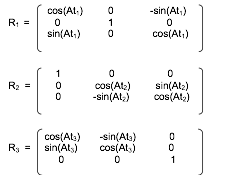
(P_Xt, P_Yt, P_Zt)^T= (R₃ · R₂ · R₁) · ((P_X, P_Y, P_Z)^T- (T_X, T_Y, T_Z)^T)

(P_Xt, P_Yt, P_Zt)_A = (136.99, -95.41, -32.48) in mm.

Step 7: Image B: Point (P_Xt, P_Yt, P_Zt)_B in Table coordinates

In this step, the table has moved from image A to image B. The table coordinates of the object of interest are the same on image A and image B because it is assumed that the patient is fixed on the table.

(P_Xt, P_Yt, P_Zt)_B = (136.99, -95.41, -32.48) in mm.

Step 8: Image B: Point (P_X, P_Y, P_Z)_B in Isocenter coordinates

In this step, the isocenter coordinates (P_X, P_Y, P_Z)_B are calculated from the table coordinates (P_Xt, P_Yt, P_Zt)_B by taking into account the table position and angles of the image B in the Isocenter coordinate system:

Tx =Table X Position to Isocenter = 20.0 mm

Ty =Table Y Position to Isocenter = 100.0 mm

Tz =Table Z Position to Isocenter = 0.0 mm

At₁ = Table Horizontal Rotation Angle = 0.0 deg

At₂ = Table Head Tilt Angle = 10.0 deg

At₃ = Table Cradle Tilt Angle = 0.0 deg

(P_X, P_Y, P_Z)^T= (R₃ · R₂ · R₁)^T· (P_Xt, P_Yt, P_Zt)^T+ (T_X, T_Y, T_Z)^T

(P_X, P_Y, P_Z)_B = (156.99, -12.11, -48.55) in mm.

Step 9: Image B: Point (P_Xp, P_Yp, P_Zp)_B in positioner coordinates

In this step, the positioner coordinates (P_Xp, P_Yp, P_Zp)_B are calculated from the isocenter coordinates (P_X, P_Y, P_Z)_B by taking into account the positioner angles of the image B in the Isocenter coordinate system:

Ap₁ = Positioner Isocenter Primary Angle = -30.0 deg

Ap₂ = Positioner Isocenter Secondary Angle = 0.0 deg

Ap₃ = Positioner Isocenter Detector Rotation Angle = 0.0 deg

(P_Xp, P_Yp, P_Zp)^T= R₃ · ((R₂ · R₁) · (P_X, P_Y, P_Z)^T)

(P_Xp, P_Yp, P_Zp)_B = (142.01, 68.00, -48.55) in mm.

Step 10: Image B: Point ( P_u, P_v)_B in positioner coordinates

In this step, the (P_u, P_v)_B coordinates in mm are calculated from the positioner coordinates (P_Xp, P_Yp, P_Zp)_B by taking into account the Distance Source to Detector and the Distance Source to Isocenter of the image B:

SID = Distance Source to Detector = 1000 mm

ISO = Distance Source to Isocenter = 800 mm

Magnification ratio = SID / (ISO - P _Yp ) = 1200/(800-68) = 1.366

Pu = P _Xp * Magnification ratio = 142.01 * 1.64 = 194.00 mm

Pv = P _Z p * Magnification ratio = -48.55 * 1.64 = -66.33 mm

( P_u, P_v)_B = (194.00, -66.33) in mm.

Step 11: Image B: Point (i, j)_B in physical detector coordinates

In this step, the physical detector coordinates (i, j)_B are calculated from the positioner coordinates ( P_u, P_v)_B by taking into account the projection of the Isocenter in physical detector coordinates, and the Detector Element Spacing of the image B:

ISO_P_idet = Position of Isocenter Projection (column) = 1024.5

ISO_P_jdet = Position of Isocenter Projection (row) = 1024.5

D_idet =Detector Element Spacing between two adjacent columns = 0.2

D_jdet =Detector Element Spacing between two adjacent rows = 0.2

i = ISO_P_idet + Pu / D_idet = 1024.5 + 194.00 / 0.2 = 1994.5

j = ISO_P_idet - Pv / D_idet = 1024.5 - (-66.33) / 0.2 = 1356.2

(i, j)_B = (1994.5, 1356.2) in detector elements.

Step 12 : Image B: Point (i, j)_B in FOV coordinates

In this step, the FOV coordinates are calculated from the physical detector coordinates by taking into account the FOV origin and the ratio between Imager Pixel Spacing and Detector Element Spacing of the image B:

D_i = Imager Pixel Spacing (column) = 0.4 mm

D_j = Imager Pixel Spacing (row) = 0.4 mm

D_idet = Detector Element Spacing between two adjacent columns = 0.2 mm

D_jdet = Detector Element Spacing between two adjacent rows = 0.2 mm

Zoom Factor (column) = D_i / D_idet = 2.0

Zoom Factor (row) = D_j / D_jdet = 2.0

FOV Origin (column) = FOV_idet = 25.0

FOV Origin (row) = FOV_jdet = 25.0

new i = (i - FOV_idet).D_idet / D_i - (1 - D_idet / D_i) / 2 = (1994.5 - 25.0) / 2.0 - 0.25 = 984.5

new j = (j - FOV_jdet).D_jdet / D_j - (1 - D_jdet / D_j) / 2 = (1356.2 - 25.0) / 2.0 - 0.25 = 665.35

(i, j)_B = (984.50, 665.35) in stored pixel data.

Step 13 : Image B: Point (i, j)_B in Pixel Data

In this step, the position (i, j)_B of the projection of the object of interest in the Pixel Data of the image B is calculated from the FOV coordinates by taking into account the FOV rotation and Horizontal Flip applied to the FOV matrix when the Pixel Data were created:

1.1: Horizontal Flip : NO

new i = i = 984.50

new j = j = 665.35

1.2: Image Rotation : 180 (clockwise)

new i = (columns -1) - i = 1000 - 1 - 984.50 = 14.50

new j = (rows -1) - j = 1000 - 1 - 665.35 = 333.65

(i, j)_B = (14.50, 333.65) in stored pixel data.

GGG Unified Worklist and Procedure Step - UPS (Informative)

GGG.1 Introduction

This section provides examples of different implementations and message sequencing when using the Unified Worklist and Procedure Step SOP Classes (UPS Push, UPS Pull, UPS Watch and UPS Event).

The examples are intended to provide a sense of how the UPS SOP Classes can be used to support a variety of workflow use cases. For the detailed specification of how the underlying DIMSE Services function, please refer to Annex CC “Unified Procedure Step Service and SOP Classes (Normative)” in PS3.4. For the detailed specification of how the RESTful services function, please refer to Section 6.9 “UPS-RS Worklist Service” in PS3.18 .

The Unified Worklist and Procedure Step Service Class combines the information that is conveyed separately by the Modality Worklist and Modality Performed Procedure Step into a single normalized object. This object is created to represent the planned step and then updated to reflect its progress from scheduled to complete and record details of the procedure performed and the results created. Additionally, the Unified Worklist supports subscription based notifications of progress and completion.

The Unified Worklist and Modality Procedure Step Service Class does not include support for complex internal task structures. It describes a single task to be performed in terms of the task request and the task results. Additional complexity is managed by the business logic.

The UPS SOP Classes define services so UPSs can be created, their status managed, notifications sent and their attributes set, queried, and retrieved. DICOM intentionally leaves open the many combinations in which these services can be implemented and applied to enact a variety of approaches to workflow.

Pull Workflow and Push Workflow

Similar to previous SOP Classes like Modality Worklist, UPS allows a performing system (using the UPS Pull SOP Class as a C-FIND SCU) to query a worklist manager (the SCP) for relevant tasks and choose which one to start working on. This is sometimes called "Pull Workflow" since the performer pulls down the list and selects an item.

UPS adds the ability for a scheduling system (using the UPS Push SOP Class as an N-CREATE SCU) to "push" a workitem onto the performing system (here an SCP). In "Push Workflow" the scheduler makes the choice of which system becomes responsible for the workitem.

Performing systems (again as an SCP) could also schedule/create their own workitems, while allowing other systems (using the UPS Watch and UPS Event SOP Classes as N-EVENT-REPORT SCUs and N-GET SCUs) to receive notifications of the activities of the performer and examine the results.

Push and Pull can also be combined in various ways. A high level departmental scheduler could break down orders and push tasks onto the acquisition worklist manager and reporting worklist manager from which modalities and reporting workstations could pull their tasks. In another scenario, a modality that has pulled an acquisition workitem off a worklist, could push a follow-up task onto a workstation to perform 3D processing or CAD on the results.

Reliable Watchers and Deletion Locks

Some UPS features (specifically the Deletion Lock - See Section CC.2.3.2, “Service Class User Behavior”) were introduced to support Reliable Watchers. By subscribing with a Deletion Lock, an SCU wishing to be a reliable watcher can signal the SCP to persist instances until the watcher has been able to retrieve final state information and remove the lock.

This means that network latency, slight delays in processing threads, or even the watcher being offline for a short time, will not prevent the watcher from reliably collecting the final state details from UPS instances it is interested in. This can be very important since the watcher may be responsible for monitoring completion of those instances, extracting details from them, and based on that and other internal logic, creating subsequent UPS Instances and populating the input data fields with information from the completed UPS. Without some form of persistence guarantee, UPS instances could disappear immediately upon entering a completed state.

Having established the Deletion Lock mechanism, it is possible that, due to equipment or processing errors, there could be cases where locks are not properly removed and some UPS instances might remain when they are no longer needed. Most SCP implementations will likely provide a way for such orphaned UPS instances to be removed under administrator control.

GGG.2 Implementation Examples

The following sections describe ways UPS workflows could be used to address some typical scenarios.

GGG.2.1 Typical SOP Class Implementations

The decision of which SOP Classes to implement in which systems will revolve partly around where it makes the most sense for the business logic to reside, what information each system would have access to, and what kind of workflow is most effective for the users.

Table GGG.1-1 shows a number of hypothetical systems and the combination of SOP Classes they might implement. For example, a typical worklist manager would support all four SOP Classes as an SCP. A typical scheduling system might want to be a UPS Push SCU to submit work items to the worklist manager, a UPS Watch SCU to subscribe for notifications and get details of the results, and a UPS Event SCU to receive the progress notifications. A simple "pull performer" might only be a UPS Pull SCU, similar to modalities today.

Other examples are listed for:

"Minimal Scheduler", a requesting system that is not interested in monitoring progress or results.
"Watcher", a system interested in tracking the progress and/or results of Unified Procedure Steps.
"General Contractor", a system that accepts work items pushed to it, then uses internal business logic to subdivide/create work items that it pushes or makes available to systems that will actually perform the work.
"Push Performer", a system, for example a CAD system, that has work pushed to it, and provides status and results information to interested observers.
"Self-Scheduled Performer", which internally schedules it's own work, but supports notifications and N-GET so the details of the work can be made available to other departmental systems.
"Self-Scheduled Pull Performer", which pushes a workitem onto a worklist manager and then pulls it off to perform it. This allows it to work on "unscheduled" procedures without taking on the responsibility of being an SCP for notifications and events.

Table GGG.1-1. SOP Classes for Typical Implementation Examples

SOP Classes	SCU				SCP
SOP Classes	UPS Push	UPS Watch	UPS Event	UPS Pull	UPS Push	UPS Watch	UPS Event	UPS Pull
Non-Performing SCUs
Minimal Scheduler	X
Typical Scheduler	X	X	X
Watcher		X	X
Worklist SCPs
Worklist Manager					X	X	X	X
General Contractor	X	X	X		X	X	X	X
Performing SCPs
Push Performer					X	X	X
Self-Scheduled Performer						X	X
Performing SCUs
Pull Performer				X
Self-Scheduled Pull Performer	X			X

A system that implements UPS Watch as an SCP will also need to implement UPS Event as an SCP to be able to send Event Reports to the systems from whom it accepts subscriptions.

GGG.2.2 Typical Pull Workflow

This example shows how a typical pull workflow could be used to manage the work of a 3D Lab. A group of 3D Workstations query a 3D Worklist Manager for work items that they perform and report their progress. In this example, the RIS would be a "Typical Scheduler", the 3D Workstation is a "Pull Performer" as seen in Table GGG.1-1 and the PACS and Modality do not implement any UPS SOP Classes.

We will assume the RIS decides which studies require 3D views and puts them on the worklist once the acquiring modality has reported it's MPPS complete. The RIS identifies the required 3D views and lists the necessary input objects in the UPS based on the image references recorded in the MPPS.

Assume the RIS has subscribed globally for all UPS instances managed by the 3D Worklist Manager.

Figure GGG.2-1. Diagram of Typical Pull Workflow

GGG.2.3 Reporting Workflow With "hand-off"

This example shows a reporting workflow with a "hand-off". Reporting Workstations query a RIS for work items to interpret/report. In this example, the RIS is a "Worklist Manager", the Reporting Workstation is both a "Pull Performer" and a "Minimal Scheduler" as shown in Table GGG.1-1 and the PACS and Modality do not implement any UPS SOP Classes. A reporting workstation claims Task X but can't complete it and "puts it back on the worklist" by canceling Task X and creating Task Y as a replacement, recording Task X as the Replaced Procedure Step.

Assume the RIS is picking up where example GGG.2.2 left off and was waiting for the 3D view generation task to be complete before putting the study on the reading worklist. The RIS identifies the necessary input objects in the UPS based on the image references recorded in the acquisition MPPS and the 3D UPS.

Figure GGG.3-1. Diagram of Reporting Workflow

You could also imagine the 3D workstation is a Mammo CAD workstation. If the first radiologist completed the report, the RIS could easily schedule Task Y as the over-read by another radiologist.

For further discussion, refer to the Section GGG.2.7 material on Hand-offs, Fail-overs and Putting Tasks Back on the Worklist.

GGG.2.4 Third Party Cancel

Cancel requests are always directed to the system managing the UPS instance since it is the SCP. When the UPS is being managed by one system (for example a Treatment Management System) and performed by a second system (for example a Treatment Delivery System), a third party would send the cancel request to the TMS and cancellation would take place as shown below.

Performing SCUs are not required to react to cancel requests, or even to listen for them, and in some situations would be unable to abort the task represented by the UPS even if they were listening. In the diagram below we assume the performing SCU is listening, willing, and able to cancel the task.

If the User had sent the cancel request while the UPS was still in the SCHEDULED state, the SCP (i.e., the TMS) could simply have canceled the UPS internally. Since the UPS state was IN PROGRESS, it was necessary to send the messages as shown. Note that since the TDS has no need for the UPS instance to persist, it subscribed without setting a Deletion Lock, and so it didn't need to bother unsubscribing later.

Figure GGG.4-1. Diagram of Third Party Cancel

GGG.2.5 Radiation Therapy Dose Calculation Push Workflow

In this example, users schedule tasks to a shared dose calculation system and need to track progress. This example is intended as a demonstration of UPS and should not be taken as prescriptive of RT Therapy procedures.

Pushing the tasks avoids problems with a pull workflow such as the server having to continually poll worklists on (a large number of) possible clients; needing to configure the server to know about all the clients; reporting results to a user who might be at several locations; and associating the results with clients automatically. Also, when performing machines each have unique capabilities, the scheduling must target individual machines, and there can be advantages for integrating the scheduling and performing activities like this.

Although not shown in the diagram, the User could have gone to a User Terminal ("Watcher") and monitored the progress from there by doing a C-FIND and selecting/subscribing to Task X.

Figure GGG.5-1. Diagram of Radiation Therapy Planning Push Workflow

In a second example, the User monitors progress from another User Terminal ("Watcher") and decides to request cancellation after 3 beams.

Figure GGG.5-2. Diagram of Remote Monitoring and Cancel

GGG.2.6 X-Ray Clinic Push Workflow

In this example, arriving patients are admitted at the RIS and sent to a specific X-Ray room for their exam.

The RIS is shown here subscribing globally for events from each Room. Alternatively the RIS could subscribe individually to each Task right after the N-CREATE is requested.

It is left open whether the patient demographics have been previously registered and the patients scheduled on the RIS or whether they are registered on the RIS when they arrive.

Figure GGG.6-1. Diagram of X-Ray Clinic Push Workflow

GGG.2.7 Other Examples

A wide variety of workflow methods are possible using the UPS SOP Classes. In addition to those diagrammed in the previous sections, a few more are briefly described here. These include examples of ways to handle unscheduled tasks, grouped tasks, append cases, "event forwarding", etc.

Self-Scheduling Push & Pull: Unscheduled and Append Cases

In radiation therapy a previously unscheduled ("emergency") procedure may be performed on a Treatment Delivery System. Normally a TDS performs scheduled procedures as a Performing SCU in a Typical Pull Workflow like that shown in GGG.2.2. A TDS that might need to perform unscheduled procedures could additionally implement UPS Push (as an SCU) and push the "unscheduled" procedure to the departmental worklist server then immediately set it IN PROGRESS as a UPS Pull SCU. The initial Push to the departmental server allows the rest of the departmental workflow to "sync up" normally to the new task on the schedule.

A modality choosing to append some additional images after the original UPS was completed could use a similar method. Since the original UPS can no longer be modified, the modality could push a new UPS instance to the Worklist Manager and then immediately set it IN PROGRESS. Many of the attribute values in the new UPS would be the same as the original UPS.

Note that for a Pull Performer that wants to handle unscheduled cases, this Push & Pull approach is pretty simple to implement. Becoming a UPS Push SCU just requires N-CREATE and N-ACTION (Request Cancel) that are quite similar to the N-SET and N-ACTION it already supports as a UPS Pull SCU.

The alternative would be implementing both UPS Watch and UPS Event as an SCP, which would be more work. Further, potential listeners would have to be aware of and monitor the performing system to track the unscheduled steps, instead of just monitoring the departmental Pull SCP.

Self-Scheduling Performer

An example of an alternative method for handling unscheduled procedures is a CAD workstation that decides for itself to perform processing on a study. By implementing UPS Watch as an SCP and UPS Event as an SCP, the workstation can create UPS instances internally and departmental systems such as the RIS can subscribe globally to the workstation to monitor its activities.

The workstation might create the UPS tasks in response to having data pushed to it, or potentially the workstation could itself also be a Watch and Event SCU and subscribe globally to relevant modality or PACS systems and watch for appropriate studies.

Push Daisy Chain

Sometimes the performer of the current task is in the best position to decide what the next task should be.

An alternative to centralized task management is daisy-chaining where each system pushes the next task to the next performer upon completion of the current task. Using a workflow similar to the X-Ray Clinic example in GGG.6, a modality could push a task to a CAD workstation to process the images created by the modality. The task would specify the necessary images and perhaps parameters relevant to the acquisition technique. The RIS could subscribe globally with the CAD workstation to track events. Another example of push daisy chain would be for the task completed at each step in a reporting process to be followed by scheduling the next logical task.

Hand-offs, Fail-overs and Putting Tasks Back on the Worklist

Sometimes the performer of the current task, after setting it to IN PROGRESS, may determine it cannot complete the task and would like the task performed by another system. It is not permitted to move the task backwards to the SCHEDULED state.

One approach is for the performer to cancel the old UPS and schedule a new UPS to be pulled off the worklist by another system or by itself at some point in the future. The new UPS would be populated with details from the original. The details of the new UPS, such as the Input Information Sequence (0040,4021), the Scheduled Workitem Code Sequence (0040,4018), and the Scheduled Processing Parameters Sequence (0074,1210), might be revised to reflect any work already completed in the old UPS. By including the "Discontinued Procedure Step rescheduled" code in the Procedure Step Discontinuation Reason Code Sequence (0074,100e) of the old UPS, the performer can allow watchers and other systems monitoring the task to know that there is a replacement for the old canceled UPS. By referencing the UID of the old UPS in the Replaced Procedure Step Sequence (0074,1224) of the new UPS, the performer can allow watchers and other systems to find the new UPS that replaced the old. A proactive SCP might even subscribe watchers of the old UPS to the new UPS that replaces it.

Alternatively, if the performer does not have the capability to create a new UPS, it could include the "Discontinued Procedure Step rescheduling recommended" code in the Procedure Step Discontinuation Reason Code Sequence (0074,100e). A very smart scheduling system could observe the cancellation reason and create the new replacement UPS as described above on behalf of the performer.

Another approach is for the performer to "sub-contract" to another system by pushing a new UPS onto that system and marking the original UPS complete after the sub-contractor finishes.

Yet another approach would be for the performer to deliver the Locking UID (by some unspecified mechanism) to another system allowing the new system to continue the work on the existing UPS. Coordination and reconciliation would be very important since the new system would need to review the current contents of the UPS, understand the current state, update the performing system information, etc.

GGG.3 Other Features

GGG.3.1 What Was Scheduled Vs. What Was Performed

The performing system for a UPS instance determines what details to put in the attributes of the Performed Procedure Information Module. It is possible that the procedure performed may differ in some details from the procedure scheduled. It is up to the performing system to decide how much the performed procedure can differ from the scheduled procedure before it is considered a different procedure, or how much must be performed before the procedure is considered complete.

In the case of cancellation, it is possible that some details of the situation may be indeterminable. Beyond meeting the Final State requirements, accurately reflecting in the CANCELED UPS instance the actual state of the task (e.g., reflecting partial work completed and/or any cleanup performed during cancellation), is at the discretion of the performing system.

In general it is expected that:

An SCU that completes a UPS differently than described in the scheduled details, but accomplishes the intended goal, would record the details as performed in the existing UPS and set it to COMPLETED. Interested systems may choose to N-GET the Performed Codes from the UPS and confirm whether they match the Scheduled Codes.
An SCU that completes part of the work described in a UPS, but does not accomplish the intended goal, would set the Performed Protocol Codes to reflect what work was fully or partially completed, set the Output Sequence to reflect the created objects and set the UPS state to CANCELED since the goal was not completed.
An SCU that completes a step with a different intent and scope in place of a scheduled UPS would cancel the original scheduled UPS, listing no work output products, and schedule a new UPS describing what was actually done, and reference the original UPS that it replaces in the Replaced Procedure Step Sequence to facilitate monitoring systems "closing the loop".
An SCU that completes multiple steps, scheduled as separate UPS instances (e.g., a dictation & a transcription & a verification), as a block would individually report each of them as completed.
An SCU that completes additional unscheduled work in the course of completing a scheduled UPS would either report additional procedure codes in the completed UPS, or create one or more new UPS instances to record the unscheduled work.

GGG.3.2 Complex Procedure Steps

There are cases where it may be useful to schedule a complex procedure that is essentially a grouping of multiple workitems. Placing multiple workitem codes in the Scheduled Workitem Code Sequence is not permitted (partly due to the additional complexities that would result related to sequencing, dependency, partial completion, etc.)

One approach is to schedule separate UPS instances for each of the component workitems and to identify the related UPS instances based on their use of a common Study UID or Order Number.

Another approach is for the site to define a single workitem code that means a pre-defined combination of what would otherwise be separate workitems, along with describing the necessary sequencing, dependencies, etc.

GGG.3.3 Gift Subscriptions

The UPS Subscription allows the Receiving AE Title to be different than the AE Title of the SCU of the N-ACTION request. This allows an SCU to sign up someone else who would be interested for a subscription. For example, a reporting workflow manager could subscribe the RIS to UPSs the reporting workflow manager creates for radiology studies, and subscribe the CIS to UPSs it creates for cardiology studies. Or a RIS could subscribe the MPPS broker or the order tracking system to the high level UPS instances and save them from having independent business logic to determine which ones are significant.

This can provide an alternative to systems using global subscriptions to stay on top of things. It also has the benefit of providing a way to avoid having to "forward" events. All interested SCUs get their events directly from the SCP. Instead of SCU A forwarding relevant events to SCU B, SCU A can simply subscribe SCU B to the relevant events.

HHH Transition from WADO to RESTful Services (Informative)

This annex discusses the design considerations that went into the definition of the WADO extension to Web and REST services.

HHH.1 Request and Response Parameters

HHH.1.1 Request Parameters

The WADO-RS and STOW-RS requests have no parameters because data is requested through well defined URLs and content negotiation through HTTP headers.

Table HHH.1-1. Summary of DICOM/Rendered URI Based WADO Parameters

Parameter	Allowed for	Requirement in Request
requestType	DICOM & Rendered	Required
studyUID	DICOM & Rendered	Required
seriesUID	DICOM & Rendered	Required
objectUID	DICOM & Rendered	Required
contentType	DICOM & Rendered	Optional
charset	DICOM & Rendered	Optional
anonymize	DICOM	Optional
annotation	Rendered	Optional
Rows, columns	Rendered	Optional
region	Rendered	Optional
windowCenter, windowWidth	Rendered	Optional
imageQuality	DICOM & Rendered	Optional
presentationUID	Rendered	Optional
presentationSeriesUID	Rendered	Optional
transferSyntax	DICOM	Optional
frameNumber	DICOM & Rendered	Optional

HHH.1.2 Response Parameters

HHH.1.2.1 URI WADO-URI

In the URI based WADO, the response is the single payload returned in the HTTP Get response. It may be the DICOM object in a DICOM format or in a rendered format.

HHH.1.2.2 Retired

See PS3.17-2017b.

HHH.1.2.3 WADO-RS

The WADO-RS Service is a transport service, as opposed to a rendering service, which provides resources that enable machine to machine transfers of binary instances, pixel data, bulk data, and metadata. These services are not primarily intended to be directly displayable in a browser.

In the REST Services implementation:

For the "DICOM Requester", one or more multipart/related parts are returned containing PS3.10 binary DICOM instances of a Study, Series, or a single Instance.
For the "Frame Pixel Data Requester", one or more multipart/related parts are returned containing the pixel data of a multi-frame SOP Instance.
For the "Bulk Data Requester", one or more multipart/related parts are returned containing the bulk data of a Study, Series or SOP Instance.
For the "Metadata Requester", an item is returned containing the XML encoded metadata selected from the retrieved objects header as described in the Native DICOM Model defined in PS3.19.

HHH.1.2.4 STOW-RS

The STOW-RS Service provides the ability to STore Over the Web using RESTful Services (i.e., HTTP based functionality equivalent to C-Store).

For the "DICOM Creator", one or more multipart/related parts are stored (posted to a STOW-RS Service) containing one or more DICOM Composite SOP Instances.
For the "Metadata and Bulk Data Creator", one or more multipart/related parts are stored (posted to a STOW-RS Service) containing the XML encoded metadata defined in PS3.19 and one or more parts containing the bulk data of a Study, Series or SOP Instance.

HHH.2 Web Services Implementation

The implementation architecture has to maximize interoperability, preserve or improve performance and minimize storage overhead.

The Web Services technologies have been selected to:

be firewall friendly and supporting security,
be supported by and interoperable between multiple development environments, and
have sufficient performance for both large and small text and for binary data.

The WADO-RS response will be provided as a list of XML and/or binary instances in a multipart/related response. The type of response depends on the media types listed in the Accept header.

The STOW-RS response is a standard HTTP status line and possibly an XML response message body. The meaning of the success, warning, or failure statuses are defined in PS3.18.

HHH.3 Uses for Web Services

HHH.3.1 General Requirements

Imaging information is important in the context of EMR/EHR. But EMR/EHR systems often do not support the DICOM protocol. The EMR/EHR vendors need access using web and web service technologies to satisfy their users.

HHH.3.2 Analysis of Use Cases

Examples of use cases / clinical scenarios, as the basis to develop the requirements, include:

Providing access to images and reports from a point-of-service application e.g., EMR.
Following references to significant images used to create an imaging report and displaying those images.
Following references / links to relevant images and imaging reports in email correspondence or clinical reports e.g., clinical summary.
Providing access to anonymized DICOM images and reports for clinical research and teaching purposes.
Providing access to a DICOM encoded imaging report associated with the DICOM IE (patient/study/series/objects) to support remote diagnostic workflows e.g., urgent medical incidents, remote consultation, clinical training, teleradiology/telemedicine applications.
Providing access to summary or selected information from DICOM objects.
Providing access to complete studies for caching, viewing, or image processing.
Storing DICOM SOP Instances using HTTP over a Network from PACS to PACS, from PACS to VNA, from VNA to VNA, from clinical application to PACS, or any other DICOM SCP.
Web clients, including mobile ones, retrieving XML and bulk data from a WADO-RS Service and adding new instances to a study.

Examples of the use cases described in 1 above are:

The EMR displays in JPEG one image with annotations on it (patient and/or technique related), based upon information provided in a report.
The EMR retrieves from a "Manifest" document all the referenced objects in DICOM and launches a DICOM viewer for displaying them (use case addressed by the IHE XDS-I.b profile).
The EMR displays in JPEG one image per series with information describing every series (e.g., series description).
The EMR displays in JPEG all the images of a series with information describing the series as well as every image (e.g., instance number and slice location for scanner images).
The EMR populates in its database for all the instances referred in a manifest (KOS) the relevant information (study ID/UID/AccessionNumber/Description/DateTime, series UID/Modality/Description/DateTime, instance UID/InstanceNumber/SliceLocation).
The EMR displays patient demographics and image slices in a browser by accessing studies through URLs that are cached and rendered in a remote data center.
A hospital transfers a DICOM Study over a network to another healthcare provider without needing special ports opened in either firewall.
A diagnostic visualization client, during post-processing, adds a series of Instances containing measurements, annotations, or reports.
A healthcare provider transfers a DICOM Study to a Patient Health Record (PHR) at the request of the patient.

As an example, the 1c use case is decomposed in the following steps (all the other use cases can be implemented through a similar sequence of basic transactions):

The EMR sends to the DICOM server the list of the objects ("selection"), asking for the object content.
The DICOM server sends back the JPEG images corresponding to the listed objects.
The EMR sends to the DICOM server the "selection" information for obtaining the relevant information about the objects retrieved.
The DICOM server sends back the corresponding information in the form of a "metadata" document, converted in XML.

HHH.3.3 Description of The Use Cases

The use cases described above in terms of clinical scenarios correspond to the following technical implementation scenarios. In each case the use is distinguished by the capabilities of the requesting system:

Does it prefer the URI based requests, or the web-services based requests.
Does it have the ability to decode and utilize the DICOM PS3.10 format or not.
Does it need the metadata describing the image and its acquisition, and/or does it need an image to be displayed.

These then become the following technical use cases.

HHH.3.3.1 URI Based WADO Use Case

The requesting system is Web Browser or other application that can make simple HTTP/HTTPS requests,
Reference information is provided as URL or similar information that can be easily converted into a URL.
The request specifies:
1. Individual SOP Instance
2. Desired format and subset selection for information to be returned
The Response provides
1. SOP instance, reformatted and subset as requested. This may be encoded as a DICOM PS3.10 instance, or rendered into a generic image format such as JPEG.

HHH.3.3.2 DICOM (Encoded Content) Requester

The requesting system is an application capable of making Web Service requests and able to process data encoded as a DICOM File, per DICOM PS3.10 encodings.
Reference information may come in a wide variety of forms. It is expected to include at least the Study UID, Series UID, and Individual SOP instance information. This may be encoded as part of an HL7 reference within a CDA document, a DICOM SOP Instance reference, or other formats.
The request specifies
1. Requested Data set
  1. Study UID
  2. List of Series UID
  3. List of SOP Instance UIDs
2. Optionally, it may also specify subset information
  1. Instance and Frame Level Retrieve SOP classes subset information for selecting frames
  2. No-pixel data request (using the Transfer Syntax parameter)
  3. Anonymization
The response provides
1. SOP Instances, encoded per DICOM PS3.10.

HHH.3.3.3 Rendered (JPEG/PDF) Requester

The requesting system: application capable of making Web Service requests. System is not capable of decoding DICOM PS3.10 formats. The system is capable of processing images in JPEG or other more generic formats.
Reference information may come in a wide variety of forms. It is expected to include at least the Study UID, Series UID, and Individual SOP instance information. This may be encoded as part of an HL7 reference within a CDA document, a DICOM SOP Instance reference, or other formats.
Request information
1. Requested Data set
  1. Study UID
  2. List of Series UID
  3. List of SOP Instance UIDs
2. Desired format and subset information
  1. JPEG/PDF/etc. selection, subset area, presentation information
  2. Frame selection for subsets of multi-frame objects
  3. What should be done for requests where image shapes and SOP classes vary and a subset is requested?
  4. Anonymize or not.
Response information
1. JPEGs
  1. Should JPEGs include tag information within the JPEG? If so, what information?
  2. How will JPEGs be related to multi-frame and multi-instance requests? Order? Tag?
2. PDFs
  1. How will PDFs be related to multi-frame and multi-instance requests? One per frame? One per instance? One for entire set?
3. Other encodings?

HHH.3.3.4 Metadata (XML Without Pixel Data, Waveform Data, etc.) Requester

The requesting system: application capable of making Web Service requests. The requesting System is not capable of decoding DICOM PS3.10 formats. The system is capable of processing metadata that describes the image, provided that the metadata is encoded in an XML format. The system can be programmed based upon the DICOM definitions for XML encoding and attribute meanings.
Reference information may come in a wide variety of forms. It is expected to include at least the Study UID, Series UID, and Individual SOP instance information. This may be encoded as part of an HL7 reference within a CDA document, a DICOM SOP Instance reference, or other formats.
Request information
1. Requested Data set
  1. Study UID
  2. List of Series UID
  3. List of SOP Instance UIDs
2. Desired format and subset information
  1. XPath definition for subset or total metadata selection
  2. What should be done when SOP classes vary and a subset is requested? The XPath will fail.
  3. Frame selection for subsets of multi-frame objects
  4. Anonymize or not.
  5. Response information
Response information
1. XML encoded metadata.

HHH.3.3.5 DICOM Requester

The requesting system is an application capable of making HTTP Service requests and able to process data encoded as a DICOM File, per DICOM PS3.10 encodings.
Requesting information for DICOM Instances may come from a wide variety of forms. It is expected to include at least the Study UID. This may be encoded as part of an HL7 reference within a CDA document, a DICOM SOP Instance reference, or other formats.
The request specifies
1. Requested Data set
  1. Study UID
2. Optionally, it may also specify subset information
  1. Series UID
  2. SOP Instance UID
The response provides
1. SOP Instances, encoded per DICOM PS3.10.

HHH.3.3.6 Frame Pixel Data Requester

The requesting system is an application capable of making HTTP requests and able to process pixel data.
Requesting information for pixel data may come in a wide variety of forms. It is expected to include at least the Study UID, Series UID, Individual SOP Instance, and Frame List information. This may be encoded as part of an HL7 reference within a CDA document, a DICOM SOP Instance reference, or other formats.
The request specifies
1. Requested Data set
  1. Study UID
  2. Series UID
  3. SOP Instance UID
  4. Frame List comprised of one or more frame numbers
The response provides pixel data

HHH.3.3.7 Bulk Data Requester

The requesting system is an application capable of making HTTP requests and able to process bulk data.
Requesting information for bulk data may come in a wide variety of forms. It is expected to include the Bulk Data URL as provided by the RetrieveMetadata resource. This may be encoded as part of an HL7 reference within a CDA document, a DICOM SOP Instance reference, or other formats.
The request specifies
1. Requested Data set
  1. Bulk Data URL
The response provides bulk data

HHH.3.3.8 Metadata Requester

The requesting system is an application capable of making HTTP requests and able to process data encoded as a XML, per DICOM PS3.19 encodings.
The Study UID may be obtained as part of an HL7 reference within a CDA document, a DICOM SOP Instance reference, or other formats.
Request information
1. Requested Data set
  1. Study UID
The response provides full study metadata encoded in XML, encoded per DICOM PS3.19.

HHH.3.3.9 DICOM Creator

The requesting system is an application capable of making HTTP Service requests and able to process data encoded as PS3.10 binary instances.
The request specifies
1. The STOW-RS Service to store POST requests.
2. Optionally, it may also specify Study Instance UID indicating all POST requests are for the indicated study.
3. SOP Instances, per DICOM PS3.10 encoding.
The response is a standard HTTP status line and an XML response message body. The meaning of the success, warning, or failure statuses are defined in PS3.18.

HHH.3.3.10 Metadata and Bulk Data Creator

The requesting system is an application capable of making HTTP requests and able to process data encoded as PS3.19 XML metadata.
The request specifies
1. The STOW-RS Service to store POST requests.
2. Optionally, it may also specify Study Instance UID indicating all POST requests are for the indicated study.
3. XML metadata, per DICOM PS3.19 encodings, and bulk data.
The response is a standard HTTP status line and an XML response message body. The meaning of the success, warning, or failure statuses are defined in PS3.18.

HHH.4 Uses For QIDO Services

HHH.4.1 General Requirements

Imaging information is important in the context of EMR/EHR. But EMR/EHR systems often do not support DICOM service classes. The EMR/EHR vendors need access using web and web service technologies to satisfy their users.

HHH.4.2 Analysis of Use Cases

Examples of use cases / clinical scenarios, used as the basis for the development of the QIDO-RS requirements, include:

Search from EMR
Populating FHIR resources
Worklist in Viewer
Study Import Duplication Check
Multiple System Query
Clinical Reconstruction
Mobile Device Access

HHH.4.2.1 Search From EMR

A General Practitioner (GP) in a clinic would like to check for imaging studies for the current patient. These studies are stored in a PACS, Vendor Neutral Archive (VNA) or HIE that supports QIDO functionality. The GP launches an Electronic Medical Record (EMR) application, and keys in the patient demographics to search for the patient record within the EMR. Once the record is open, the EMR, using QIDO, makes requests to the back-end systems, supplying Patient ID (including issuer) and possibly other parameters (date of birth, date range, modality, etc.). That system returns the available studies along with meta-data for each study that will help the GP select the study to open. The meta-data would include, but is not limited to, Study Description, Study Date, Modality, and Referring Physician.

HHH.4.2.2 Populating FHIR Resources

HL7 has introduced FHIR (Fast Healthcare Interoperability Resources) as a means of providing access to healthcare informatics information using RESTful web services.

While FHIR will not replicate the information contained in a PACS or other medical imaging storage system, it is desirable for FHIR to present a view of the medical imaging studies available for a particular patient along with the means of retrieving the imaging data using other RESTful services.

HHH.4.2.3 Worklist in Viewer

A Radiologist, is reading studies in the office, using software that maintains diagnostic orders for the facility. This system produces the radiology worklist of studies to be read and provides meta-data about each scheduled procedure, including the Study Instance UID. When the next study is selected to be read on the worklist, the system, using the Study Instance UID, makes a QIDO request to the local archive to discover the instances and relevant study meta-data associated with the procedure to display. Subsequent QIDO requests are made to the local archive and to connected VNA archives to discover candidate relevant prior studies for that patient.

For each candidate relevant prior, the full study metadata will be retrieved using WADO-RS and processed to generate the list of relevant priors.

HHH.4.2.4 Multiple Systems Query

A Radiologist is working in a satellite clinic, which has a system with QIDO functionality and small image cache. The main hospital with which the clinic is affiliated has a system with QIDO functionality and a large historical image archive or VNA. The viewing software displays a worklist of patients, and a study is selected for viewing. The viewer checks for prior studies, by making QIDO requests to both the local cache and remote archive using the Patient ID, Name and Date of Birth, if available. If the Patient Identifier isn't available, other means (such as by other demographics, or a Master Patient Index) could be utilized. Any studies that meet relevant prior criteria can be pre-fetched.

HHH.4.2.5 Clinical Reconstruction

A Neurologist is preparing a surgical plan for a patient with a brain tumor using three-dimensional reconstruction software, which takes CT images and builds a 3D model of various structures. After supplying the patient demographics (or Patient Identifier), the software requests a list of appropriate studies for reconstruction (based on Study Date, Body Region and Modality). Once the user has selected a study and series, the software contacts the QIDO server again, requesting the SOP Instance UIDs of all images of a certain thickness (specified in specific DICOM tags) and frame of reference to be returned. The software then uses this information to retrieve, using the WADO-RS service, the appropriate DICOM objects needed to prepare the rendered volume for display.

HHH.4.2.6 Mobile Device Access

A General Practitioner (GP) has left the medical ward for a few hours, and is paged with a request to look at a patient X-Ray image in order to grant a discharge. The GP carries a smart phone that has been pre-loaded with credentials and secured. The device makes a QIDO request to the server, to look for studies from the last hour that list the GP as the Referring Physician. The GP is able to retrieve and view the matching studies, and can make a determination whether to return to the ward for further review or to sign the discharge order using the phone.

HHH.4.3 Description of The Use Cases

Does it prefer XML or JSON results?
Does it need to perform searches at the Series and Instance level or can it process the full Study metadata?
What attributes does it need to search against?
What attributes does it need for each matching Study, Series or Composite Instance?

These questions can be applied to the use cases:

Search from EMR
1. JSON or XML
2. Study
3. Study Instance UID, Patient ID
4. Accession Number, Issuer of Accession Number, Study Description, Study Date, Modality, Number of Series, Number of Instances
Populating FHIR resources
1. JSON or XML
2. Study, Series and Instance
3. Patient ID and Issuer of Patient ID
4. All attributes required by the FHIR Imaging Study Resource (see http://www.hl7.org/implement/standards/fhir/imagingstudy.htm)
Worklist in Viewer
1. JSON or XML
2. Study
3. Study Instance UID, Patient ID, Issuer of Patient ID
4. Series Instance UIDs, SOP Instance UIDs, patient demographics, Study Description, Study Date, Modality, Referring Physician
Study Import Duplication Check
1. JSON or XML
2. Study
3. Study Instance UID, Series Instance UID, SOP Instance UID
4. Study Instance UID
Multiple System Query
1. JSON or XML
2. Study
3. Patient ID, Issuer of Patient ID, Patient Name, Patient Date of Birth
4. Study Instance UID, Accession Number, Study Description, Study Date, Modalities in Study
Clinical Reconstruction
1. JSON or XML
2. Study, Series, Instance
3. Study Instance UID, Series Instance UID
4. SOP Instance UID, Image Instance Level Attributes
Mobile Device Access
1. JSON
2. Study, Series and Instance
3. Patient ID, Issuer of Patient ID, Patient Name, Patient Date of Birth, Study Date, Referring Physician
4. Instance Date/time, Modalities in Study

These then become the following technical use cases.

HHH.4.3.1 XML Study Search Use Case

The requesting web-based application can make QIDO-RS requests, parse XML and then make WADO-RS requests
The request specifies:
1. Multipart XML
2. Search parameters, including:
  1. Patient ID
  2. Issuer of Patient ID
  3. Patient Name
  4. Study Description
  5. Study Date
  6. Modalities in Study
  7. Referring Physician
  8. etc.
The Response provides
1. One PS3.19 XML NativeDicomModel element for each matching Study
2. All requested DICOM attributes for each matching Study
3. WADO-RS Retrieve URL for each matching Study
The requesting system identifies the Studies of interest and uses WADO-RS to retrieve data

HHH.4.3.2 XML Study, Series and Instance Search Use Case

The requesting system is a simple web-based application that can make QIDO-RS requests and parse XML and then make WADO URL requests
The request specifies:
1. Multipart XML
2. Search parameters, including:
  1. Patient ID
  2. Issuer of Patient ID
  3. Patient Name
  4. Patient Date of Birth
  5. Study Description
  6. Study Date
  7. Modalities in Study
  8. Referring Physician
The Response provides
1. One PS3.19 XML NativeDicomModel element for each matching Study
2. All requested DICOM attributes for each matching Study
The requesting system identifies the Study of interest and uses Search For Series to identify a series of interest
[repeat B-D for Series, Instance]
The requesting system uses WADO URL to retrieve specific instances

HHH.4.3.3 JSON Use Case

The requesting system is a mobile application that can make QIDO-RS requests, parse JSON and then make WADO URL requests.
The request specifies:
1. JSON
2. Search parameters, including:
  1. Patient ID
  2. Issuer of Patient ID
  3. Patient Name
  4. Patient Date of Birth
  5. Study Description
  6. Study Date
  7. Modalities in Study
  8. Referring Physician
The Response provides
1. One DICOM JSON element containing all matching Studies
2. All requested DICOM attributes for each matching Study
The requesting system identifies the Study of interest and uses Search For Series to identify a series of interest
[repeat B-D for Series, Instance]
The requesting system uses WADO URL to retrieve specific instances

HHH.5 Retired

See PS3.17-2017b.

HHH.6 Retired

See PS3.17-2017b.

HHH.7 Uses for Server Options Services

Clients would like to be able to discover a list of devices that support DICOM RESTful services and query a DICOM RESTful service to determine which options are supported, such as:

Supported services and transactions
Supported Transfer Syntaxes and Media Types
Supported Accept header values
Supported query parameters

HHH.7.1 WADL Example (XML)

The following WADL XML example contains all the required elements for an origin-server that supports WADO-RS, QIDO-RS and STOW-RS with all required services and parameters.

<application xsi:schemaLocation="http://wadl.dev.java.net/2009/02 wadl.xsd"
             xmlns:xsd="http://www.w3.org/2001/XMLSchema"
             xmlns="http://wadl.dev.java.net/2009/02">
 <resources base="http://medical.examplehospital.org/dicomweb">
  <resource path="studies">
   <method name="GET" id="SearchForStudies">
    <request>
     <param name="Accept" style="header"
            default="type=application/dicom+json">
      <option value="multipart/related; type=application/dicom+xml" />
      <option value="application/dicom+json" />
     </param>
     <param name="Cache-control" style="header">
      <option value="no-cache" />
     </param>
     <param name="limit" style="query" />
     <param name="offset" style="query" />
     <param name="StudyDate" style="query" />
     <param name="00080020" style="query" />
     <param name="StudyTime" style="query" />
     <param name="00080030" style="query" />
     <param name="AccessionNumber" style="query" />
     <param name="00080050" style="query" />
     <param name="ModalitiesInStudy" style="query" />
     <param name="00080061" style="query" />
     <param name="ReferringPhysicianName" style="query" />
     <param name="00080090" style="query" />
     <param name="PatientName" style="query" />
     <param name="00100010" style="query" />
     <param name="PatientID" style="query" />
     <param name="00100020" style="query" />
     <param name="StudyInstanceUID" style="query" repeating="true" />
     <param name="0020000D" style="query" repeating="true" />
     <param name="StudyID" style="query" />
     <param name="00200010" style="query" />
     <param name="includefield" style="query" repeating="true">
      <option value="all" />
     </param>
    </request>
    <response status="200">
     <param name="Warning" style="header"
            fixed="299 {SERVICE}: The fuzzymatching parameter is not supported.
            Only literal matching has been performed." />
     <representation mediaType="multipart/related; type=application/dicom+xml" />
     <representation mediaType="application/dicom+json" />
    </response>
    <response status="400 401 403 413 503" />
   </method>
   <method name="POST" id="StoreInstances">
    <request>
     <param name="Accept" style="header" default="application/dicom+xml">
      <option value="application/dicom+xml" />
     </param>
     <representation mediaType="multipart/related; type=application/dicom" />
     <representation mediaType="multipart/related; type=application/dicom;
                                          transfer-syntax=1.2.840.10008.1.2.1" />
     <representation mediaType="multipart/related; type=application/dicom+xml" />
    </request>
    <response status="202 409">
     <representation mediaType="application/dicom+xml" />
    </response>
    <response status="400 401 403 503" />
   </method>
   <resource path="{StudyInstanceUID}">
    <method name="GET" id="RetrieveStudy">
     <request>
      <param name="Accept" style="header"
                 default="multipart/related; type=application/dicom">
       <option value="multipart/related; type=application/dicom" />
       <option value="multipart/related; type=application/dicom;
                                          transfer-syntax=1.2.840.10008.1.2.1" />
       <option value="multipart/related; type=application/octet-stream" />
      </param>
     </request>
     <response status="200 206">
      <representation mediaType="multipart/related; type=application/dicom" />
      <representation mediaType="multipart/related; type=application/dicom;
                                          transfer-syntax=1.2.840.10008.1.2.1" />
      <representation mediaType="multipart/related; type=application/octet-stream" />
     </response>
     <response status="400 404 406 410 503"></response>
    </method>
    <method name="POST" id="StoreStudyInstances">
     <request>
      <param name="Accept" style="header" default="application/dicom+xml">
       <option value="application/dicom+xml" />
      </param>
      <representation mediaType="multipart/related; type=application/dicom" />
      <representation mediaType="multipart/related; type=application/dicom;
                                          transfer-syntax=1.2.840.10008.1.2.1" />
      <representation mediaType="multipart/related; type=application/dicom+xml" />
     </request>
     <response status="202 409">
      <representation mediaType="application/dicom+xml" />
     </response>
     <response status="400 401 403 503" />
    </method>
    <resource path="series">
     <method name="GET" id="SearchForStudySeries">
      <request>
       <param name="Accept" style="header"
                  default="type=application/dicom+json">
        <option value="multipart/related; type=application/dicom+xml" />
        <option value="application/dicom+json" />
       </param>
       <param name="Cache-control" style="header">
        <option value="no-cache" />
       </param>
       <param name="limit" style="query" />
       <param name="offset" style="query" />
       <param name="Modality" style="query" />
       <param name="00080060" style="query" />
       <param name="SeriesInstanceUID" style="query" repeating="true" />
       <param name="0020000E" style="query" repeating="true" />
       <param name="SeriesNumber" style="query" />
       <param name="00200011" style="query" />
       <param name="PerformedProcedureStepStartDate" style="query" />
       <param name="00400244" style="query" />
       <param name="PerformedProcedureStepStartTime" style="query" />
       <param name="00400245" style="query" />
       <param name="RequestAttributeSequence" style="query" />
       <param name="00400275" style="query" />
       <param name="RequestAttributeSequence.ScheduledProcedureStepID" style="query" />
       <param name="00400275.00400009" style="query" />
       <param name="RequestAttributeSequence.RequestedProcedureID" style="query" />
       <param name="00400275.00401001" style="query" />
       <param name="includefield" style="query" repeating="true">
        <option value="all" />
       </param>
      </request>
      <response status="200">
       <param name="Warning" style="header"
              fixed="299 {SERVICE}: The fuzzymatching parameter is not supported.
              Only literal matching has been performed." />
       <representation mediaType="multipart/related; type=application/dicom+xml" />
       <representation mediaType="application/dicom+json" />
      </response>
      <response status="400 401 403 413 503" />
     </method>
     <resource path="{SeriesInstanceUID}">
      <method name="GET" id="RetrieveSeries">
       <request>
        <param name="Accept" style="header"
                 default="multipart/related; type=application/dicom">
         <option value="multipart/related; type=application/dicom" />
         <option value="multipart/related; type=application/dicom;
                                          transfer-syntax=1.2.840.10008.1.2.1" />
         <option value="multipart/related; type=application/octet-stream" />
        </param>
       </request>
       <response status="200 206">
        <representation mediaType="multipart/related; type=application/dicom" />
        <representation mediaType="multipart/related; type=application/dicom;
                                          transfer-syntax=1.2.840.10008.1.2.1" />
        <representation mediaType="multipart/related; type=application/octet-stream" />
       </response>
       <response status="400 404 406 410 503"></response>
      </method>
      <resource path="instances">
       <method name="GET" id="SearchForStudySeriesInstances">
        <request>
         <param name="Accept" style="header"
                default="type=application/dicom+json">
          <option value="multipart/related; type=application/dicom+xml" />
          <option value="application/dicom+json" />
         </param>
         <param name="Cache-control" style="header">
          <option value="no-cache" />
         </param>
         <param name="limit" style="query" />
         <param name="offset" style="query" />
         <param name="SOPClassUID" style="query" repeating="true" />
         <param name="00080016" style="query" repeating="true" />
         <param name="SOPInstanceUID" style="query" repeating="true" />
         <param name="00080018" style="query" repeating="true" />
         <param name="InstanceNumber" style="query" />
         <param name="00200013" style="query" />
         <param name="includefield" style="query" repeating="true">
          <option value="all" />
         </param>
        </request>
        <response status="200">
         <param name="Warning" style="header"
                fixed="299 {SERVICE}: The fuzzymatching parameter is not supported.
                Only literal matching has been performed." />
         <representation mediaType="multipart/related; type=application/dicom+xml" />
         <representation mediaType="application/dicom+json" />
        </response>
        <response status="400 401 403 413 503" />
       </method>
       <resource path="{SOPInstanceUID}">
        <method name="GET" id="RetrieveInstance">
         <request>
          <param name="Accept" style="header"
                 default="multipart/related; type=application/dicom">
           <option value="multipart/related; type=application/dicom" />
           <option value="multipart/related; type=application/dicom;
                                          transfer-syntax=1.2.840.10008.1.2.1" />
           <option value="multipart/related; type=application/octet-stream" />
          </param>
         </request>
         <response status="200 206">
          <representation mediaType="multipart/related; type=application/dicom" />
          <representation mediaType="multipart/related; type=application/dicom;
                                          transfer-syntax=1.2.840.10008.1.2.1" />
          <representation mediaType="multipart/related; type=application/octet-stream" />
         </response>
         <response status="400 404 406 410 503"></response>
        </method>
        <resource path="frames">
         <resource path="{framelist}">
          <method name="GET" id="RetrieveFrames">
           <request>
            <param name="Accept" style="header"
                   default="multipart/related; type=application/octet-stream">
             <option value="multipart/related; type=application/octet-stream" />
            </param>
           </request>
           <response status="200">
            <representation mediaType="multipart/related; type=application/octet-stream" />
           </response>
           <response status="400 404 406 410 503"></response>
          </method>
         </resource>
        </resource>
        <resource path="metadata">
         <method name="GET" id="RetrieveInstanceMetadata">
          <request>
           <param name="Accept" style="header"
                  default="type=application/dicom+json">
            <option value="multipart/related; type=application/dicom+xml" />
            <option value="application/dicom+json" />
           </param>
          </request>
          <response status="200">
           <representation mediaType=" multipart/related; type=application/dicom+xml" />
          </response>
          <response status="400 404 406 410 503"></response>
         </method>
        </resource>
       </resource>
      </resource>
      <resource path="metadata">
       <method name="GET" id="RetrieveSeriesMetadata">
        <request>
         <param name="Accept" style="header"
                  default="type=application/dicom+json">
          <option value="multipart/related; type=application/dicom+xml" />
          <option value="application/dicom+json" />
         </param>
        </request>
        <response status="200">
         <representation mediaType="multipart/related; type=application/dicom+xml" />
        </response>
        <response status="400 404 406 410 503"></response>
       </method>
      </resource>
     </resource>
    </resource>
    <resource path="instances">
     <method name="GET" id="SearchForStudyInstances">
      <request>
       <param name="Accept" style="header"
                  default="type=application/dicom+json">
        <option value="multipart/related; type=application/dicom+xml" />
        <option value="application/dicom+json" />
       </param>
       <param name="Cache-control" style="header">
        <option value="no-cache" />
       </param>
       <param name="limit" style="query" />
       <param name="offset" style="query" />
       <param name="SOPClassUID" style="query" />
       <param name="00080016" style="query" />
       <param name="SOPInstanceUID" style="query" repeating="true" />
       <param name="00080018" style="query" repeating="true" />
       <param name="Modality" style="query" />
       <param name="00080060" style="query" />
       <param name="SeriesInstanceUID" style="query" repeating="true" />
       <param name="0020000E" style="query" repeating="true" />
       <param name="SeriesNumber" style="query" />
       <param name="00200011" style="query" />
       <param name="InstanceNumber" style="query" />
       <param name="00200013" style="query" />
       <param name="PerformedProcedureStepStartDate" style="query" />
       <param name="00400244" style="query" />
       <param name="PerformedProcedureStepStartTime" style="query" />
       <param name="00400245" style="query" />
       <param name="RequestAttributeSequence" style="query" />
       <param name="00400275" style="query" />
       <param name="RequestAttributeSequence.ScheduledProcedureStepID" style="query" />
       <param name="00400275.00400009" style="query" />
       <param name="RequestAttributeSequence.RequestedProcedureID" style="query" />
       <param name="00400275.00401001" style="query" />
       <param name="includefield" style="query" repeating="true">
        <option value="all" />
       </param>
      </request>
      <response status="200">
       <param name="Warning" style="header"
              fixed="299 {SERVICE}: The fuzzymatching parameter is not supported.
              Only literal matching has been performed." />
       <representation mediaType="multipart/related; type=application/dicom+xml" />
       <representation mediaType="application/dicom+json" />
      </response>
      <response status="400 401 403 413 503" />
     </method>
    </resource>
    <resource path="metadata">
     <method name="GET" id="RetrieveStudyMetadata">
      <request>
       <param name="Accept" style="header"
                  default="type=application/dicom+json">
        <option value="multipart/related; type=application/dicom+xml" />
        <option value="application/dicom+json" />
       </param>
      </request>
      <response status="200">
       <representation mediaType="multipart/related; type=application/dicom+xml" />
      </response>
      <response status="400 404 406 410 503"></response>
     </method>
    </resource>
   </resource>
  </resource>
  <resource path="series">
   <method name="GET" id="SearchForSeries">
    <request>
     <param name="Accept" style="header"
                  default="type=application/dicom+json">
      <option value="multipart/related; type=application/dicom+xml" />
      <option value="application/dicom+json" />
     </param>
     <param name="Cache-control" style="header">
      <option value="no-cache" />
     </param>
     <param name="limit" style="query" />
     <param name="offset" style="query" />
     <param name="StudyDate" style="query" />
     <param name="00080020" style="query" />
     <param name="StudyTime" style="query" />
     <param name="00080030" style="query" />
     <param name="AccessionNumber" style="query" />
     <param name="00080050" style="query" />
     <param name="Modality" style="query" />
     <param name="00080060" style="query" />
     <param name="ModalitiesInStudy" style="query" />
     <param name="00080061" style="query" />
     <param name="ReferringPhysicianName" style="query" />
     <param name="00080090" style="query" />
     <param name="PatientName" style="query" />
     <param name="00100010" style="query" />
     <param name="PatientID" style="query" />
     <param name="00100020" style="query" />
     <param name="StudyInstanceUID" style="query" repeating="true" />
     <param name="0020000D" style="query" repeating="true" />
     <param name="SeriesInstanceUID" style="query" />
     <param name="0020000E" style="query" />
     <param name="StudyID" style="query" />
     <param name="00200010" style="query" />
     <param name="SeriesNumber" style="query" />
     <param name="00200011" style="query" />
     <param name="PerformedProcedureStepStartDate" style="query" />
     <param name="00400244" style="query" />
     <param name="PerformedProcedureStepStartTime" style="query" />
     <param name="00400245" style="query" />
     <param name="RequestAttributeSequence" style="query" />
     <param name="00400275" style="query" />
     <param name="RequestAttributeSequence.ScheduledProcedureStepID" style="query" />
     <param name="00400275.00400009" style="query" />
     <param name="RequestAttributeSequence.RequestedProcedureID" style="query" />
     <param name="00400275.00401001" style="query" />
     <param name="includefield" style="query" repeating="true">
      <option value="all" />
     </param>
    </request>
    <response status="200">
     <param name="Warning" style="header"
            fixed="299 {SERVICE}: The fuzzymatching parameter is not supported.
            Only literal matching has been performed." />
     <representation mediaType="multipart/related; type=application/dicom+xml" />
     <representation mediaType="application/dicom+json" />
    </response>
    <response status="400 401 403 413 503" />
   </method>
   <resource path="{SeriesInstanceUID}">
    <resource path="instances">
     <method name="GET" id="SearchForSeriesInstances">
      <request>
       <param name="Accept" style="header"
                  default="type=application/dicom+json">
        <option value="multipart/related; type=application/dicom+xml" />
        <option value="application/dicom+json" />
       </param>
       <param name="Cache-control" style="header">
        <option value="no-cache" />
       </param>
       <param name="limit" style="query" />
       <param name="offset" style="query" />
       <param name="SOPClassUID" style="query" repeating="true" />
       <param name="00080016" style="query" repeating="true" />
       <param name="SOPInstanceUID" style="query" repeating="true" />
       <param name="00080018" style="query" repeating="true" />
       <param name="InstanceNumber" style="query" />
       <param name="00200013" style="query" />
       <param name="includefield" style="query" repeating="true">
        <option value="all" />
       </param>
      </request>
      <response status="200">
       <param name="Warning" style="header"
              fixed="299 {SERVICE}: The fuzzymatching parameter is not supported.
              Only literal matching has been performed." />
       <representation mediaType="application/dicom+json" />
       <representation mediaType="multipart/related; type=application/dicom+xml" />
      </response>
      <response status="400 401 403 413 503" />
     </method>
    </resource>
   </resource>
  </resource>
  <resource path="instances">
   <method name="GET" id="SearchForInstances">
    <request>
     <param name="Accept" style="header"
                  application/dicom+json">
      <option value="multipart/related; type=application/dicom+xml" />
      <option value="application/dicom+json" />
     </param>
     <param name="Cache-control" style="header">
      <option value="no-cache" />
     </param>
     <param name="limit" style="query" />
     <param name="offset" style="query" />
     <param name="SOPClassUID" style="query" repeating="true" />
     <param name="00080016" style="query" repeating="true" />
     <param name="SOPInstanceUID" style="query" repeating="true" />
     <param name="00080018" style="query" repeating="true" />
     <param name="StudyDate" style="query" />
     <param name="00080020" style="query" />
     <param name="StudyTime" style="query" />
     <param name="00080030" style="query" />
     <param name="AccessionNumber" style="query" />
     <param name="00080050" style="query" />
     <param name="Modality" style="query" />
     <param name="00080060" style="query" />
     <param name="ModalitiesInStudy" style="query" />
     <param name="00080061" style="query" />
     <param name="ReferringPhysicianName" style="query" />
     <param name="00080090" style="query" />
     <param name="PatientName" style="query" />
     <param name="00100010" style="query" />
     <param name="PatientID" style="query" />
     <param name="00100020" style="query" />
     <param name="StudyInstanceUID" style="query" repeating="true" />
     <param name="0020000D" style="query" repeating="true" />
     <param name="SeriesInstanceUID" style="query" repeating="true" />
     <param name="0020000E" style="query" repeating="true" />
     <param name="SeriesNumber" style="query" />
     <param name="00200011" style="query" />
     <param name="InstanceNumber" style="query" />
     <param name="00200013" style="query" />
     <param name="PerformedProcedureStepStartDate" style="query" />
     <param name="00400244" style="query" />
     <param name="PerformedProcedureStepStartTime" style="query" />
     <param name="00400245" style="query" />
     <param name="RequestAttributeSequence" style="query" />
     <param name="00400275" style="query" />
     <param name="RequestAttributeSequence.ScheduledProcedureStepID" style="query" />
     <param name="00400275.00400009" style="query" />
     <param name="RequestAttributeSequence.RequestedProcedureID" style="query" />
     <param name="00400275.00401001" style="query" />
     <param name="includefield" style="query" repeating="true">
      <option value="all" />
     </param>
    </request>
    <response status="200">
     <param name="Warning" style="header"
            fixed="299 {SERVICE}: The fuzzymatching parameter is not supported.
            Only literal matching has been performed." />
     <representation mediaType="multipart/related; type=application/dicom+xml" />
     <representation mediaType="application/dicom+json" />
    </response>
    <response status="400 401 403 413 503" />
   </method>
  </resource>
  <resource path="{BulkDataURL}">
   <method name="GET" id="RetrieveBulkData">
    <request>
     <param name="Accept" style="header"
            default="multipart/related; type=application/octet-stream">
      <option value="multipart/related; type=application/octet-stream" />
     </param>
    </request>
    <response status="200">
     <representation mediaType="multipart/related; type=application/octet-stream" />
    </response>
    <response status="400 404 406 410 503"></response>
   </method>
  </resource>
 </resources>
</application>

III Ophthalmic Thickness Map Use Cases (Informative)

III.1 Introduction

Several ophthalmic devices produce thickness and/or height measurements of certain anatomical features of the posterior eye (e.g., optic nerve head topography, retinal thickness map, etc.). The measurements are mapped topographically as monochromatic images with pseudo color maps, and used extensively for diagnostic purposes by clinicians.

III.2 Macular Retinal Thickness Example

Quantitative ophthalmic OCT image analysis provides essential thickness measurement data of the retina. In the clinical practice two thickness parameters are commonly used: total retinal thickness (TR) in macular region and retinal nerve fiber layer thickness (RNFL) in optic nerve head (ONH) region. TR is widely applied to assess various retinal pathologies involving macula (e.g., cystoid macular edema, age-related macular degeneration, macular hole, etc.). The RNFL thickness measurement is most commonly used for glaucoma assessment.

Figure III.2-1 is an example of 2D TR map computed on a 3D OCT cube data from a healthy eye. The color bar on the left provides a color-to-thickness representation to allow interpretation of the false color coded 2D thickness map in the middle. The image on the right shows one OCT frame representing a retinal cross section along the red line (across the middle of the thickness map). TR is defined as the thickness between internal limiting membrane (white line on the OCT frame on the right) and RPE/Choroid interface (blue line on the OCT frame). These two borders are automatically detected using a segmentation algorithm applied to the entire 3D volume.

Figure III.2-1. Macular Example Mapping

III.3 RNFL Example

Figure III.3-1 is an example of a 2D RNFL map computed on a 3D OCT cube data from a healthy eye. The figure layout is the same as the previous example. The RNFL thickness is limited to the thickness of this single layer of the retina that is comprised of the ganglion cell axons that course to the optic nerve head and exit the eye as the optic nerve. Note that this image depicts a BMP mask in the center of the map where the optic nerve head (ONH) exists and no RNFL measurements can be obtained. In this example, the mask is displayed as a black area, which does not contain any thickness information (not zero micron thickness). Since the color bar representation is not relevant at the ONH, common practice is to mask it to avoid confusion or misinterpretation due to meaningless thickness data in this area.

Figure III.3-1. RNFL Example Mapping

III.4 Diabetic Macular Edema Example

A 48 year old Navajo male with diabetes, decreased visual acuity and fundoscopic stigmata of diabetic retinopathy receives several tests to assess his likelihood of macular edema. Optical coherence tomography (OPT) is performed to assess the thickness of the retina in the macular area. This is performed with retinal thickness depicted by ophthalmic mapping. The results is an Ophthalmic Thickness Map SOP instance with the Ophthalmic Thickness Mapping Type Code Sequence (0022,1436) set to "Absolute Ophthalmic Thickness" and the Measurements Units Code Sequence (0040,08EA) in the Real World Value Mapping Macro, set to "micrometer". The OPT image is also referenced in attribute Referenced Instance Sequence (0008,114A).

Figure III.4-1. Macula Edema Thickness Map Example

Since the thickness of the macula varies normally based upon a number of dependencies such as age, gender, race, etc. Interpretation of the retinal thickness in any given patient may be done in the context of normative data that accounts for these variables. The thickness data used to generate the thickness map is analyzed using a manufacturer specific algorithm for comparison to normative data relevant to this specific patient. The results of this analysis is depicted on a second thickness "map" (second SOP Instance) showing each pixel's variation from normal in terms of confidence that the variation is real and not due to chance. Specific confidence levels are then depicted by arbitrary color mapping registered to the fundus photograph. This is typically noted as the percent probability that the variation is abnormal e.g., p >5%, p <5%, p <1% etc. The results is an Ophthalmic Thickness Map SOP instance with the Ophthalmic Thickness Mapping Type Code Sequence (0022,1436) set to "Thickness deviation category from normative data". Mapping the "categories" to a code concept is accomplished via Attribute Pixel Value Mapping to Coded Concept Sequence (0022,1450).

Figure III.4-2. Macula Edema Probability Map Example

III.5 Glaucoma Example

A patient was presented with normal visual acuity OU (both eyes), intraocular pressures (IOP) of 18 mm Hg OU (both eyes), and 0.7 C/D OD (right eye) and 0.6 C/D ratio OS (left eye). Corneal pachymetry showed slight thinning in both eyes at 523µ OD (right eye) and 530µ OS (left eye). Static threshold perimetry testing showed nonspecific defects OU (both eyes) and was unreliable due to multiple fixation losses. Confocal scanning laser ophthalmoscopy produced OPM topographic representations of both optic nerves suggestive of glaucoma. The contouring of the optic nerve head (ONH) in the left eye showed a slightly enlarged cup with diffuse thinning of the superior neural rim. In the right eye, there was greater enlargement of the cup and sloping of the cup superior-temporally with a clear notch of the neural rim at the 12:30 position. Corneal compensated scanning laser polarimetry was performed bilaterally. Analysis of the OPM representation of the retinal nerve fiber layer (RNFL) thickness map showed moderate retinal nerve fiber loss with accentuation at the superior pole bilaterally. The patient was diagnosed with normal tension glaucoma and started on a glaucoma medication. Follow-up examinations showed stable reduction in his IOP to 11 mm Hg OU (both eyes) and no further progression of his ONH or RNFL defects.

III.6 Retinal Thickness Definition

Using OCT technology, there are typically 2 major highly reflective bands generally visible; inner and outer highly reflective bands (IHRB and OHRB).

The inner band corresponds to the inner portion of the retina, which consists of ILM (internal limiting membrane), RNFL (retinal nerve fiber layer), GCL (ganglion cell layer), IPL (inner plexiform layer), INL (inner nuclear layer), and OPL (outer plexiform layer). In terms of the reflectivity, they present a high-low-high-low-high pattern, in general. Presumably RNFL, IPL, and OPL are the highly reflective layers and GCL and INL are of low reflectivity. ILM itself may or may not be visible in OCT images (depending on the scanning beam incidence angle), but for convenience it is used to label the vitreo-retinal interface.

The outer band is considered as the RPE (retinal pigment epithelium) /Choroid complex that consist of portion of photoreceptor, RPE, Bruch's membrane, and portion of choroid. Within the RPE/Choroid complex, there are 3 highly reflective interfaces identifiable, presumably corresponding to IS/OS (photoreceptor inner/out segment junction), RPE, and Bruch's membrane.

Clinically 3 retinal thickness measurements are generally acknowledged and utilized; RNFL thickness, GCC (ganglion cell complex) thickness, and total retinal thickness.

RNFL thickness is defined as the distance between ILM and outer interface of the inner most highly reflective layer presumably RNFL.

GCC thickness is defined as the distance between ILM and the outer interface of the second inner highly reflective layer presumably the outer border of inner plexiform layer (IPL).

Total retinal thickness definition varies among OCT manufacturers. The classic definition is the distance between ILM and the first highly reflective interface (presumably IS-OS) in the OHRB (Total retinal thickness (ILM to IS-OS) ). A second definition is the distance between ILM and the second highly reflective interface (presumably RPE) in the OHRB (Total retinal thickness (ILM to RPE) ). A third definition is the distance between ILM and the third highly reflective interface (presumably Bruch's membrane) in the OHRB (Total retinal thickness (ILM to BM) ).

Figure III.6-1. Observable Layer Structures

III.7 Thickness Calculations Between Various Devices

When interpreting quantitative data obtained from imaging devices, comparing may be an issue. Using different devices manufactured by different companies usually ends up with non-comparable measurements because they use different optics and different algorithms to make measurements.

Currently there are multiple SD-OCT devices independently manufactured, and data comparability has become problematic. When patients change doctors or otherwise receive care from more than one provider, previously acquired data may occur on different devices and become almost useless simply because the present doctor has no access to the same device. Another problem occurs with longitudinal assessments on the same device after it has undergone upgrade to a newer generation. In this case new baseline measurements must be obtained due to incomparability of the data (this happens even for the same make different generation devices). Attempts to normalize the measurements have been unsuccessful.

The manufacturer, model, serial number, and software version information are available in the Equipment Module, and is very important for considering the significant importance of the information to the quantitative data between various SOP Instances.

JJJ Optical Surface Scan

JJJ.1 General Information

When supporting textures within one acquisition process, multiple series are generated. There is one Series containing the Surfaces and another containing the textures. References are used to link Instances in different series together.

Figure JJJ.1-1. Optical Surface Scan Relationships

JJJ.2 One Single Shot Without Texture Acquisition As Point Cloud

Use cases: A single surface record of a patient is made, for example teeth, nose, or breast. If third party software does the post-processing only the point cloud needs to be stored.

The Surface Scan Point Cloud instance will be used because a point cloud is stored. A study with a single series is created.

Figure JJJ.2-1. One Single Shot Without Texture Acquisition As Point Cloud

JJJ.3 One Single Shot With Texture Acquisition As Mesh

Use cases: A scanner device providing triangulated objects with textures, e.g., for documentation of burns or virtual autopsy.

The Surface Scan Mesh instance will be used because a triangulated object is stored. A study with two series will be created. One series contains a Surface Mesh instance and the other series a VL Photographic Image instance. The latter stores the texture, which is mapped on the surface mesh and is linked to the Surface Scan Mesh instance via the UV Mapping Sequence (0080,0008).

Figure JJJ.3-1. One Single Shot With Texture Acquisition As Mesh

JJJ.4 Storing Modified Point Cloud With Texture As Mesh

Use cases: The surface of a textured object has been modified, for example artifacts have been manually removed after the study or surgery. The new result is stored.

In the study of the origin Surface Scan Point Cloud instance a Surface Scan Mesh instance is created in its own series containing the modified mesh. The Referenced Surface Data Sequence (0080,0013) will be used to reference the original instance. The mesh as well as the point cloud points to the texture using the Referenced Surface Data Sequence (0080,0012).

Figure JJJ.4-1. Storing Modified Point Cloud With Texture As Mesh

JJJ.5 Multishot Without Texture As Point Clouds and Merged Mesh

Use-case: Objects, which need to be scanned from multiple points of view, such as the nose.

After the acquired point clouds have been merged by a post-processing software application, the calculated surface mesh is stored in the same study in a new series. The Referenced Surface Data Sequence (0080,0013) points to all origin Surface Scan Point Cloud instances that have been used for reconstruction. The Registration Method Code Sequence (0080,0003) is used to indicate that multiple point clouds have been merged.

Figure JJJ.5-1. Multishot Without Texture As Point Clouds and Merged Mesh

JJJ.6 Multishot With Two Texture Per Point Cloud

Use-case: In the application field of dental procedures some products support switching between two different textures for the same surface.

In this case a number of VL Photographic Image instances are stored in the same series.

The UV Mapping Sequence (0080,0008) is used to associate the VL Photographic Image instances with the Surface Scan Point Cloud instance. The Texture Label (0080,0009) is used to identify the textures of one point cloud.

Figure JJJ.6-1. Multishot With Two Texture Per Point Cloud

JJJ.7 Using Colored Vertices Instead of Texture

Use-case: A single surface record of a patient is made, for example teeth, nose, or breast. If third party software does the post-processing only the point cloud needs to be stored. Gray or color values can be assigned to each point in the point cloud.

The point cloud is stored in a Surface Scan Point Cloud instance. A study with a single series is created. One or both of the attributes Surface Point Presentation Value Data (0080,0006), or Surface Point Color CIELab Value Data (0080,0007) may be used to assign gray or color values to each point in the point cloud.

Figure JJJ.7-1. Using Colored Vertices Instead of Texture

JJJ.8 4D Surface Data Analysis

Use-case: To replay a sequence of multiple 3D shots of different facial expressions of a patient before facial surgeries such as facial transplantation.

A time stamp for each shot is stored in the Acquisition DateTime attribute (0008,002A).

JJJ.9 Referencing A Texture From Another Series

Use-case: A texture from another series must be applied to a point cloud.

The Referenced Instances And Access Macro is used within the Referenced Textures Sequence (0080,0012) to reference a VL Photographic Image instance from a different study.

Figure JJJ.9-1. Referencing A Texture From Another Series

KKK Use-cases For Conversion of Classic Single Frame Images to Legacy Converted Enhanced Multi-frame Images (Informative)

KKK.1 Introduction

Traditionally, images from cross-sectional modalities like CT, MR and PET have been stored with one reconstructed slice in a single frame instance. Large studies with a large number of slices potentially pose a problem for many existing implementations, both for efficient transfer from the central store to the user's desktop for viewing or analysis, and for bulk transfer between two stores (e.g., between a PACS and another archive or a regional image repository).

There are two primary issues:

Transporting large numbers of slices as separate single instances (files) is potentially extremely inefficient due to the overhead associated with each transfer (such as C-STORE acknowledgment and database insertion).
Replicating the Attributes describing the entire patient/study/series/acquisition in every separate single instance is also potentially extremely inefficient, and though the size of the this information is trivial by comparison with the bulk data, the effort to repeatedly parse it and sort out what it means as a whole on the receiving end is not trivial.

The Enhanced family of modality-specific multi-frame IODs is intended to address both these concerns, but there is a large installed base of older equipment that does not yet support these, both on the sending and receiving end, and a large archive of single frame instances.

An interim step, a legacy transition strategy for a mixed environment containing older and newer modalities, PACS and workstations, is described here. It is predicated on the ability to "convert" single frame instances into new "enhanced multi-frame instances".

KKK.2 Enhanced Legacy Converted Image Storage IODs

The Enhanced family of modality-specific multi-frame IODs contain many requirements that cannot be satisfied by the limited information typically available in the older single frame objects. A family of Multi-frame Secondary Capture IODs is available, but their use would mean that a recipient could not depend on the presence of important cross-sectional information like spacing, position and orientation. Accordingly, a new family of modality-specific Legacy Converted Enhanced Image Storage IODs has been defined that bridge the gap in conversion complexity and usability between these two extremes.

KKK.3 Heterogeneous Environment

Figure KKK-1 illustrates the approach to enabling a heterogeneous environment with conversion from single to multi-frame objects as appropriate. In this figure, modalities that generate single or enhanced images peacefully co-exist with PACS or workstations that support either or both.

Figure KKK-1. Heterogeneous environment with conversion between single and multi-frame objects

The following use-cases are explicitly supported:

A PACS that accepts single frame images, and converts them to multi-frame images for its own internal use.
A PACS that accepts single frame images, and converts them to multi-frame images for externalization via DICOM services (Query/Retrieval) so that they can be used by external workstations (or other processing applications) that support multi-frame images.
A PACS that accepts multi-frame images from a modality, and converts them to single frame images for its own internal use.
A PACS that accepts true and/or legacy converted enhanced multi-frame images, and converts them to single frame images for externalization via DICOM services (Query/Retrieval) so that they can be used by external workstations (or other processing applications) that do not support multi-frame images.
A modality that can create true enhanced multi-frame images, as well as receive true (+/- legacy converted) enhanced multi-frame images.
Return of results from workstations in either single frame or true or legacy converted enhanced multi-frame form.

The amount of standard information is the same in single frame and transitional legacy-converted multi-frame images, but greater in the true enhanced multi-frame images, and this affects the level of functionality obtainable within the PACS or with an external workstation (without depending on private information).

Since the transitional legacy-converted and true enhanced multi-frame images share a common structure and common functional group macros, this scalability can be implemented incrementally.

It is NOT the expectation that modalities will generate Legacy Converted Enhanced Image Storage SOP Instances; rather, they should create True Enhanced Image Storage SOP Instances fully populated with the appropriate standard attributes and codes.

KKK.4 Compatibility With Modality Association Negotiation

This strategy is compatible with an approach commonly implemented on acquisition modalities when deciding which SOP Class to use to encode images.

Normally a modality will propose in the Association that images be transferred using the SOP Class for which the IOD provides the richest set of information (i.e., the True Enhanced Image Storage SOP Class), and will choose the corresponding Abstract Syntax for C-STORE Operations if the Association Acceptor accepts multiple choices of SOP Class.

Consider a modality that supports the appropriate modality-specific Enhanced Image Storage SOP Class, but which is faced with the dilemma of a PACS that does not. In this case, it will commonly "fall back" to sending images the "old" way as single-frame SOP Class Instances, either because it has been pre-configured that way by service personnel, or because it discovers this limitation during Association Negotiation. This strategy is also common amongst modalities for which there are different choices of single frame SOP Class (e.g., DX versus CR versus Secondary Capture, for Digital X-Rays). In some cases, this may be implemented formally using the ability during Association Negotiation to specify a Related General SOP Class (Section B.4.2.1 “SCU Fall-Back Behavior” in PS3.4 ).

If the PACS is upgraded to include multi-frame conversion capability, and no change is made in the configuration of the modality, or in the SOP Classes accepted by the PACS, then in this scenario, the PACS can potentially convert the single-frame instances into Legacy Converted Enhanced instances. The net result is continuing sacrifice of information compared to what the modality is actually capable of.

A better choice, since the PACS is now capable of handling multi-frame images, is to also reconfigure it to also accept the "true" Enhanced Image rather than just "transitional" Legacy Converted Enhanced Storage SOP Classes. Since the two SOP Class families use the same structure and common important Functional Groups, in all likelihood the PACS will be able to use either class of objects, and in a future upgrade take advantage of the additional information in the superior object (perhaps for more complex processing or annotation or rendering). In any case, storing the modality's best output in the archive will benefit future re-use as priors and may enable greater functionality in external workstations.

A special consideration is when prior images need to be displayed on the modality before starting a new study (perhaps to setup a comparable protocol or better understand the request). In this case, care needs to be taken with respect to which images are accessible to the modality (either pushed to it or retrieved by it), and the question of "round trip fidelity" of conversion arises.

KKK.5 Query and Retrieval

The coexistence (either actually or logically) of two different representations of the same information creates a potential challenge in that the user must not be presented with both sets simultaneously.

A naïve conversion that added converted images to the study without an ability to distinguish or "filter" them from view would not only be confusing but would potentially result in twice as much data to transfer.

Accordingly, the Query/Retrieve mechanism is extended with an optional extended negotiation capability to specify which "view" of the information is required by the SCU:

A "classic" view, which includes either original (as received) classic single frame images or enhanced multi-frame images converted to single frame.
An "enhanced" view, which includes either original (as received) enhanced multi-frame images, or classic single frame images converted to true or legacy converted enhanced multi-frame.

KKK.6 Referential Integrity

Often instances within a Study will cross-reference each other. For example, a Presentation State or a Structured Report or an RT Structure Set will reference the images to which they apply, cross-sectional images may reference localizer images, and images that were acquired with annotations may contain references to Presentation States encoding those annotations.

Accordingly, when there are multiple "views" of the same study content (classic or enhanced), the instances will have different SOP Instance and Series Instance UIDs for converted content in each view. Hence any references within an instance to a converted instance needs to be updated as well. In doing such an update of references to UIDs, instances that might not otherwise have needed to be converted do need to be converted, and so on, until the entire set of instances within the scope of the conversion for the view has referential integrity.

In practice, the only instances that do not need to be converted (and assigned new UIDs) are those that contain no references and are not classic or enhanced images to be converted.

Whether or not assignment of a converted instance to a new Series triggers the need to convert all instances in that Series to the new Series, even if they would not otherwise be converted, is not defined (i.e., it is neither required nor prohibited, and hence a Series can be "split" as a consequence of conversion).

The scope of referential integrity required is defined to be the Patient. Instances in one Study may be referenced from another (e.g., as prior images).

KKK.7 Persistence and Determinism

The rules for conversion specify that the SOP Instance and Series Instance UIDs of converted images be changed, and that the same UIDs be used each time that a query or retrieval is performed. The strict separation of the two "views" of the same information, coupled with the "determinism" that results in the same identification and organization of each view every time, are required for stability across successive operations.

Were this not to be the case, for example, the results of a query (C-FIND) might be different from the results of a subsequent retrieval (C-MOVE or C-GET), or for that matter, successive queries. Further, references to specific instance UID in either view may be recorded in external systems (e.g., in an EMR), hence it is important that these remain stable and accessible.

This places a burden on the Q/R SCP to either retain a record of the mapping of UIDs from one view to the other, or to use some deterministic process that results in the same UIDs (one could envisage some hashing scheme, for instance). How this is implemented is beyond the scope of the standard to define. The determinism requirement does not remove the uniqueness requirement; in particular it is not appropriate to attempt to derive new UIDs by adding a suffix to a UID generated by a different application, for example.

There is no time limit placed on the determinism; it is expected to be indefinite, at least within the control of the system. This is a factor that should be taken into account both in the design of federated Q/R SCPs that may integrate subsidiary SCPs that support this mechanism. It should also be considered during migration to a new Q/R SCP, which ideally should support the mechanism, and should support the same mapping from one view to another as was provided by the Q/R SCP being migrated. This may be non-trivial, since the algorithm for conversion may be different between the two systems. It may be necessary to define some persistent, standard, serialized mapping of one set of UIDs to the other.

KKK.8 Source References

It is also useful to save references in converted SOP instances to their source. Accordingly, converted instances are required to contain such references, both for image conversions as well as for ancillary instances that may be updated, such as Presentation States and Structured Reports.

Obviously, the references to the source instances for the conversion are excluded from conversion themselves. If the instances have been converted on different systems, however, there is a possibility that the source references will be "replaced" and a record of the "chain" of multiple conversions will not be persisted.

There is no mechanism to define forward references in the source to the converted instances, since that would imply changing the source instances from their original form, and while this is acceptable within the scope of the normal "coercion" that a Storage SCP is permitted to perform, it is probably not sufficiently useful to justify the effort. This does imply some asymmetry however, depending on the direction of conversion (classic to enhanced or vice versa); only one set will contain the references.

In performing round trip conversion, without access to the source instances, the referenced source UIDs can be used as the UIDs for the newly created converted instances.

KKK.9 Uncertainty Principle

When does a converted view come into existence? By definition, when it is "observed". However, a practical question is when to start conversion. A Study is never, theoretically, complete, yet the semantics for conversion and consistency are defined at the Study level.

Another practical question is whether or not to make the received instances available, even though the converted ones may not yet have been created.

In the absence of the concept of "study completion" in DICOM, no firm rules can be defined. However, in practice, most systems have an internal "completion" concept, which may or may not be related to the completion of the Performed Procedure Steps that are related to the sets of instances in question, or may be established through some other mechanism, such as operator intervention, possibly via a RIS message (e.g., after QC checks are signed off as complete, or after a Study has been declared as "ready to read").

A system may elect to "dynamically" begin conversion as instances arrive and update the information in the conversion as new instances are encountered, or it may wait until some state is established that allows it to perform the conversion "statically". In either case, the information in the converted view via the query/retrieval mechanisms should be immutable once made available. I.e., once a conversion has been "distributed", it would be desirable for the system to block subsequent changes to the Study, except to the extent that there is a need for correction and management of errors (in which case mechanisms such as IHE Image Object Change Management (IOCM) may be appropriate).

LLL Conversion of Single Frame Images to Legacy Converted Enhanced Multi-frame Images (Informative)

LLL.1 Introduction

LLL.2 Simple CT Example

In this example, two consecutive transverse CT slices encoded as CT Image SOP Class Instances are shown, with a Grayscale Softcopy Presentation State reference to one of them, compared to the converted Legacy Converted Enhanced CT Image SOP Class Instance and a revised Grayscale Softcopy Presentation State that applies to it.

LLL.2.1 Images

LLL.2.1.1 First Slice As Classic Image

Nesting	Attribute	Tag	VR	VL (hex)	Value
	Specific Character Set	(0008,0005)	CS	000a	ISO_IR 100
	Image Type	(0008,0008)	CS	0016	ORIGINAL\PRIMARY\AXIAL
	Instance Creation Date	(0008,0012)	DA	0008	20061230
	Instance Creation Time	(0008,0013)	TM	0006	094053
	SOP Class UID	(0008,0016)	UI	001a	1.2.840.10008.5.1.4.1.1.2
	SOP Instance UID	(0008,0018)	UI	003c	1.3.6.1.4.1.9328.50.1.21169049221871725649891126757390969029
	Study Date	(0008,0020)	DA	0008	20061230
	Content Date	(0008,0023)	DA	0008	20061230
	Study Time	(0008,0030)	TM	0006	100000
	Content Time	(0008,0033)	TM	0000
	Accession Number	(0008,0050)	SH	0010	2263295914110886
	Modality	(0008,0060)	CS	0002	CT
	Manufacturer	(0008,0070)	LO	0000
	Referring Physician's Name	(0008,0090)	PN	0000
	Patient's Name	(0010,0010)	PN	0008	277654^
	Patient ID	(0010,0020)	LO	0010	RIDER-2357766186
	Patient's Birth Date	(0010,0030)	DA	0008	19301018
	Patient's Sex	(0010,0040)	CS	0000
	Patient Identity Removed	(0012,0062)	CS	0004	YES
	De-identification Method	(0012,0063)	LO	002a	CTP: DICOM-S142-Baseline: 20090627:021422
	Contrast/Bolus Agent	(0018,0010)	LO	0000
	Body Part Examined	(0018,0015)	CS	0006	CHEST
	Scan Options	(0018,0022)	CS	000c	HELICAL MODE
	Slice Thickness	(0018,0050)	DS	0008	1.250000
	KVP	(0018,0060)	DS	0004	120
	Data Collection Diameter	(0018,0090)	DS	000a	500.000000
	Reconstruction Diameter	(0018,1100)	DS	000a	375.000000
	Distance Source to Detector	(0018,1110)	DS	000a	949.075012
	Distance Source to Patient	(0018,1111)	DS	000a	541.000000
	Gantry/Detector Tilt	(0018,1120)	DS	0008	0.000000
	Table Height	(0018,1130)	DS	000a	170.500000
	Rotation Direction	(0018,1140)	CS	0002	CW
	Exposure Time	(0018,1150)	IS	0004	500
	X-Ray Tube Current	(0018,1151)	IS	0004	298
	Exposure	(0018,1152)	IS	0002	4
	Filter Type	(0018,1160)	SH	000c	BODY FILTER
	Generator Power	(0018,1170)	IS	0006	36000
	Focal Spot(s)	(0018,1190)	DS	0008	0.700000
	Convolution Kernel	(0018,1210)	SH	0004	LUNG
	Patient Position	(0018,5100)	CS	0004	FFS
	Revolution Time	(0018,9305)	FD	0008	0.5
	Single Collimation Width	(0018,9306)	FD	0008	0.625
	Total Collimation Width	(0018,9307)	FD	0008	40
	Table Speed	(0018,9309)	FD	0008	78.75
	Table Feed per Rotation	(0018,9310)	FD	0008	39.375
	Spiral Pitch Factor	(0018,9311)	FD	0008	0.984375
	Contributing Equipment Sequence	(0018,a001)	SQ	ffffffff
%item
	Manufacturer	(0008,0070)	LO	0008	Acme Corp
	Contribution DateTime	(0018,a002)	DT	0018	20110710084725.070-0400
	Contribution Description	(0018,a003)	ST	0016	Merged patient context
	Purpose of Reference Code Sequence	(0040,a170)	SQ	ffffffff
%item
	Code Value	(0008,0100)	SH	0006	109103
	Coding Scheme Designator	(0008,0102)	SH	0004	DCM
	Code Meaning	(0008,0104)	LO	0014	Modifying Equipment
%enditem
%endseq
%enditem
%endseq
	Study Instance UID	(0020,000d)	UI	003e	1.3.6.1.4.1.9328.50.1.331429121990566779475389049484716775937
	Series Instance UID	(0020,000e)	UI	003e	1.3.6.1.4.1.9328.50.1.160525591228102999616019562758104412505
	Study ID	(0020,0010)	SH	0004	1234
	Series Number	(0020,0011)	IS	0002	8
	Acquisition Number	(0020,0012)	IS	0002	1
	Instance Number	(0020,0013)	IS	0002	43
	Image Position (Patient)	(0020,0032)	DS	0022	-197.899994\-195.800003\-81.750000
	Image Orientation (Patient)	(0020,0037)	DS	0036	1.000000\0.000000\0.000000\0.000000\1.000000\0.000000
	Frame of Reference UID	(0020,0052)	UI	003c	1.3.6.1.4.1.9328.50.1.69905286559358212664901756199898527044
	Position Reference Indicator	(0020,1040)	LO	0002	SN
	Slice Location	(0020,1041)	DS	000a	-81.750000
	Samples per Pixel	(0028,0002)	US	0002	0001
	Photometric Interpretation	(0028,0004)	CS	000c	MONOCHROME2
	Rows	(0028,0010)	US	0002	0200
	Columns	(0028,0011)	US	0002	0200
	Pixel Spacing	(0028,0030)	DS	0012	0.732422\0.732422
	Bits Allocated	(0028,0100)	US	0002	0010
	Bits Stored	(0028,0101)	US	0002	0010
	High Bit	(0028,0102)	US	0002	000f
	Pixel Representation	(0028,0103)	US	0002	0001
	Pixel Padding Value	(0028,0120)	SS	0002	f830
	Window Center	(0028,1050)	DS	0002	40
	Window Width	(0028,1051)	DS	0004	400
	Rescale Intercept	(0028,1052)	DS	0006	-1024
	Rescale Slope	(0028,1053)	DS	0002	1
	Rescale Type	(0028,1054)	LO	0002	HU
	Performed Procedure Step Start Date	(0040,0244)	DA	0008	20061230
	Performed Procedure Step Start Time	(0040,0245)	TM	0006	092119
	Private Creator	(01F1,0010)	LO	0008	ACMEVEND
	Private Acme Acquisition Type	(01F1,1001)	CS	0006	SPIRAL
	Private Acme Scan Parameter	(01F1,1002)	FL	0006	39.2

LLL.2.1.2 Second Slice As Classic Image

Nesting	Attribute	Tag	VR	VL (hex)	Value
	Specific Character Set	(0008,0005)	CS	000a	ISO_IR 100
	Image Type	(0008,0008)	CS	0016	ORIGINAL\PRIMARY\AXIAL
	Instance Creation Date	(0008,0012)	DA	0008	20061230
	Instance Creation Time	(0008,0013)	TM	0006	094053
	SOP Class UID	(0008,0016)	UI	001a	1.2.840.10008.5.1.4.1.1.2
	SOP Instance UID	(0008,0018)	UI	003e	1.3.6.1.4.1.9328.50.1.118458571690318148036673922876743615666
	Study Date	(0008,0020)	DA	0008	20061230
	Content Date	(0008,0023)	DA	0008	20061230
	Study Time	(0008,0030)	TM	0006	100000
	Content Time	(0008,0033)	TM	0000
	Accession Number	(0008,0050)	SH	0010	2263295914110886
	Modality	(0008,0060)	CS	0002	CT
	Manufacturer	(0008,0070)	LO	0000
	Referring Physician's Name	(0008,0090)	PN	0000
	Patient's Name	(0010,0010)	PN	0008	277654^
	Patient ID	(0010,0020)	LO	0010	RIDER-2357766186
	Patient's Birth Date	(0010,0030)	DA	0008	19301018
	Patient's Sex	(0010,0040)	CS	0000
	Patient Identity Removed	(0012,0062)	CS	0004	YES
	De-identification Method	(0012,0063)	LO	002a	CTP: DICOM-S142-Baseline: 20090627:021422
	Contrast/Bolus Agent	(0018,0010)	LO	0000
	Body Part Examined	(0018,0015)	CS	0006	CHEST
	Scan Options	(0018,0022)	CS	000c	HELICAL MODE
	Slice Thickness	(0018,0050)	DS	0008	1.250000
	KVP	(0018,0060)	DS	0004	120
	Data Collection Diameter	(0018,0090)	DS	000a	500.000000
	Reconstruction Diameter	(0018,1100)	DS	000a	375.000000
	Distance Source to Detector	(0018,1110)	DS	000a	949.075012
	Distance Source to Patient	(0018,1111)	DS	000a	541.000000
	Gantry/Detector Tilt	(0018,1120)	DS	0008	0.000000
	Table Height	(0018,1130)	DS	000a	170.500000
	Rotation Direction	(0018,1140)	CS	0002	CW
	Exposure Time	(0018,1150)	IS	0004	500
	X-Ray Tube Current	(0018,1151)	IS	0004	298
	Exposure	(0018,1152)	IS	0002	4
	Filter Type	(0018,1160)	SH	000c	BODY FILTER
	Generator Power	(0018,1170)	IS	0006	36000
	Focal Spot(s)	(0018,1190)	DS	0008	0.700000
	Convolution Kernel	(0018,1210)	SH	0004	LUNG
	Patient Position	(0018,5100)	CS	0004	FFS
	Revolution Time	(0018,9305)	FD	0008	0.5
	Single Collimation Width	(0018,9306)	FD	0008	0.625
	Total Collimation Width	(0018,9307)	FD	0008	40
	Table Speed	(0018,9309)	FD	0008	78.75
	Table Feed per Rotation	(0018,9310)	FD	0008	39.375
	Spiral Pitch Factor	(0018,9311)	FD	0008	0.984375
	Contributing Equipment Sequence	(0018,a001)	SQ	ffffffff
%item
	Manufacturer	(0008,0070)	LO	0008	Acme Corp
	Contribution DateTime	(0018,a002)	DT	0018	20110710084722.235-0400
	Contribution Description	(0018,a003)	ST	0016	Merged patient context
	Purpose of Reference Code Sequence	(0040,a170)	SQ	ffffffff
%item
	Code Value	(0008,0100)	SH	0006	109103
	Coding Scheme Designator	(0008,0102)	SH	0004	DCM
	Code Meaning	(0008,0104)	LO	0014	Modifying Equipment
%enditem
%endseq
%enditem
%endseq
	Study Instance UID	(0020,000d)	UI	003e	1.3.6.1.4.1.9328.50.1.331429121990566779475389049484716775937
	Series Instance UID	(0020,000e)	UI	003e	1.3.6.1.4.1.9328.50.1.160525591228102999616019562758104412505
	Study ID	(0020,0010)	SH	0004	1234
	Series Number	(0020,0011)	IS	0002	8
	Acquisition Number	(0020,0012)	IS	0002	1
	Instance Number	(0020,0013)	IS	0002	42
	Image Position (Patient)	(0020,0032)	DS	0022	-197.899994\-195.800003\-80.500000
	Image Orientation (Patient)	(0020,0037)	DS	0036	1.000000\0.000000\0.000000\0.000000\1.000000\0.000000
	Frame of Reference UID	(0020,0052)	UI	003c	1.3.6.1.4.1.9328.50.1.69905286559358212664901756199898527044
	Position Reference Indicator	(0020,1040)	LO	0002	SN
	Slice Location	(0020,1041)	DS	000a	-80.500000
	Samples per Pixel	(0028,0002)	US	0002	0001
	Photometric Interpretation	(0028,0004)	CS	000c	MONOCHROME2
	Rows	(0028,0010)	US	0002	0200
	Columns	(0028,0011)	US	0002	0200
	Pixel Spacing	(0028,0030)	DS	0012	0.732422\0.732422
	Bits Allocated	(0028,0100)	US	0002	0010
	Bits Stored	(0028,0101)	US	0002	0010
	High Bit	(0028,0102)	US	0002	000f
	Pixel Representation	(0028,0103)	US	0002	0001
	Pixel Padding Value	(0028,0120)	SS	0002	f830
	Window Center	(0028,1050)	DS	0002	40
	Window Width	(0028,1051)	DS	0004	400
	Rescale Intercept	(0028,1052)	DS	0006	-1024
	Rescale Slope	(0028,1053)	DS	0002	1
	Rescale Type	(0028,1054)	LO	0002	HU
	Performed Procedure Step Start Date	(0040,0244)	DA	0008	20061230
	Performed Procedure Step Start Time	(0040,0245)	TM	0006	092119
	Private Creator	(01F1,0010)	LO	0008	ACMEVEND
	Private Acme Acquisition Type	(01F1,1001)	CS	0006	SPIRAL
	Private Acme Scan Parameter	(01F1,1002)	FL	0006	40.1

LLL.2.1.3 Legacy Converted Enhanced Image Containing Both Slices

Nesting	Attribute	Tag	VR	VL (hex)	Value
	Image Type	(0008,0008)	CS	001c	ORIGINAL\PRIMARY\AXIAL\NONE
	Instance Creation Date	(0008,0012)	DA	0008	20061230
	Instance Creation Time	(0008,0013)	TM	0006	094053
	SOP Class UID	(0008,0016)	UI	0016	1.2.840.10008.5.1.4.1.1.2.2
	SOP Instance UID	(0008,0018)	UI	003a	1.3.6.1.4.1.5962.99.1.2830.2144.1344607895685.1.1.1234.8.1
	Study Date	(0008,0020)	DA	0008	20061230
	Content Date	(0008,0023)	DA	0008	20061230
	Study Time	(0008,0030)	TM	0006	100000
	Content Time	(0008,0033)	TM	0000
	Accession Number	(0008,0050)	SH	0010	2263295914110886
	Modality	(0008,0060)	CS	0002	CT
	Manufacturer	(0008,0070)	LO	0000
	Referring Physician's Name	(0008,0090)	PN	0000
	Pixel Presentation	(0008,9205)	CS	000a	MONOCHROME
	Volumetric Properties	(0008,9206)	CS	0006	VOLUME
	Volume Based Calculation Technique	(0008,9207)	CS	0004	NONE
	Query/Retrieve View	(0008,0053)	CS	0008	ENHANCED
	Patient's Name	(0010,0010)	PN	0008	277654^
	Patient ID	(0010,0020)	LO	0010	RIDER-2357766186
	Patient's Birth Date	(0010,0030)	DA	0008	19301018
	Patient's Sex	(0010,0040)	CS	0000
	Patient Identity Removed	(0012,0062)	CS	0004	YES
	De-identification Method	(0012,0063)	LO	002a	CTP: DICOM-S142-Baseline: 20090627:021422
	Body Part Examined	(0018,0015)	CS	0006	CHEST
	Patient Position	(0018,5100)	CS	0004	FFS
	Content Qualification	(0018,9004)	CS	0008	PRODUCT
	Contributing Equipment Sequence	(0018,a001)	SQ	ffffffff
%item
	Manufacturer	(0008,0070)	LO	0008	Acme Corp
	Contribution DateTime	(0018,a002)	DT	0018	20110710084722.235-0400
	Contribution Description	(0018,a003)	ST	0016	Merged patient context
	Purpose of Reference Code Sequence	(0040,a170)	SQ	ffffffff
%item
	Code Value	(0008,0100)	SH	0006	109103
	Coding Scheme Designator	(0008,0102)	SH	0004	DCM
	Code Meaning	(0008,0104)	LO	0014	Modifying Equipment
%enditem
%endseq
%enditem
%item
	Manufacturer	(0008,0070)	LO	0008	PixelMed
	Institution Name	(0008,0080)	LO	0008	PixelMed
	Institution Address	(0008,0081)	ST	000a	Bangor, PA
	Institutional Department Name	(0008,1040)	LO	0014	Software Development
	Manufacturer's Model Name	(0008,1090)	LO	0028	com.pixelmed.dicom.SetWithEnhancedImages
	Software Version(s)	(0018,1020)	LO	0022	Vers. Fri Aug 10 06:56:43 EDT 2012
	Contribution DateTime	(0018,a002)	DT	0018	20120810101135.692-0400
	Contribution Description	(0018,a003)	ST	0032	Legacy Enhanced Image created from Classic Images
	Purpose of Reference Code Sequence	(0040,a170)	SQ	ffffffff
%item
	Code Value	(0008,0100)	SH	0006	109106
	Coding Scheme Designator	(0008,0102)	SH	0006	DCM
	Code Meaning	(0008,0104)	LO	002a	Enhanced Multi-frame Conversion Equipment
%enditem
%endseq
%enditem
%endseq
	Study Instance UID	(0020,000d)	UI	003e	1.3.6.1.4.1.9328.50.1.331429121990566779475389049484716775937
	Series Instance UID	(0020,000e)	UI	0038	1.3.6.1.4.1.5962.99.1.2830.2144.1344607895685.1.3.1234.8
	Study ID	(0020,0010)	SH	0004	1234
	Series Number	(0020,0011)	IS	0002	8
	Instance Number	(0020,0013)	IS	0002	1
	Frame of Reference UID	(0020,0052)	UI	003c	1.3.6.1.4.1.9328.50.1.69905286559358212664901756199898527044
	Position Reference Indicator	(0020,1040)	LO	0002	SN
	Samples per Pixel	(0028,0002)	US	0002	0001
	Photometric Interpretation	(0028,0004)	CS	000c	MONOCHROME2
	Number of Frames	(0028,0008)	IS	0002	2
	Rows	(0028,0010)	US	0002	0200
	Columns	(0028,0011)	US	0002	0200
	Bits Allocated	(0028,0100)	US	0002	0010
	Bits Stored	(0028,0101)	US	0002	0010
	High Bit	(0028,0102)	US	0002	000f
	Pixel Representation	(0028,0103)	US	0002	0001
	Pixel Padding Value	(0028,0120)	SS	0002	f830
	Burned In Annotation	(0028,0301)	CS	0002	NO
	Lossy Image Compression	(0028,2110)	CS	0002	00
	Performed Procedure Step Start Date	(0040,0244)	DA	0008	20061230
	Performed Procedure Step Start Time	(0040,0245)	TM	0006	092119
	Acquisition Context Sequence	(0040,0555)	SQ	ffffffff
%endseq
	Presentation LUT Shape	(2050,0020)	CS	0008	IDENTITY
	Shared Functional Groups Sequence	(5200,9229)	SQ	ffffffff
%item
	CT Image Frame Type Sequence	(0018,9329)	SQ	ffffffff
%item
	Frame Type	(0008,9007)	CS	001c	ORIGINAL\PRIMARY\AXIAL\NONE
	Pixel Presentation	(0008,9205)	CS	000a	MONOCHROME
	Volumetric Properties	(0008,9206)	CS	0006	VOLUME
	Volume Based Calculation Technique	(0008,9207)	CS	0004	NONE
%enditem
%endseq
	Plane Orientation Sequence	(0020,9116)	SQ	ffffffff
%item
	Image Orientation (Patient)	(0020,0037)	DS	0036	1.000000\0.000000\0.000000\0.000000\1.000000\0.000000
%enditem
%endseq
	Unassigned Shared Converted Attributes Sequence	(0020,9170)	SQ	ffffffff
%item
	Scan Options	(0018,0022)	CS	000c	HELICAL MODE
	KVP	(0018,0060)	DS	0004	120
	Data Collection Diameter	(0018,0090)	DS	000a	500.000000
	Reconstruction Diameter	(0018,1100)	DS	000a	375.000000
	Distance Source to Detector	(0018,1110)	DS	000a	949.075012
	Distance Source to Patient	(0018,1111)	DS	000a	541.000000
	Gantry/Detector Tilt	(0018,1120)	DS	0008	0.000000
	Table Height	(0018,1130)	DS	000a	170.500000
	Rotation Direction	(0018,1140)	CS	0002	CW
	Exposure Time	(0018,1150)	IS	0004	500
	X-Ray Tube Current	(0018,1151)	IS	0004	298
	Exposure	(0018,1152)	IS	0002	4
	Filter Type	(0018,1160)	SH	000c	BODY FILTER
	Generator Power	(0018,1170)	IS	0006	36000
	Focal Spot(s)	(0018,1190)	DS	0008	0.700000
	Convolution Kernel	(0018,1210)	SH	0004	LUNG
	Revolution Time	(0018,9305)	FD	0008	0.5
	Single Collimation Width	(0018,9306)	FD	0008	0.625
	Total Collimation Width	(0018,9307)	FD	0008	40
	Table Speed	(0018,9309)	FD	0008	78.75
	Table Feed per Rotation	(0018,9310)	FD	0008	39.375
	Spiral Pitch Factor	(0018,9311)	FD	0008	0.984375
	Acquisition Number	(0020,0012)	IS	0002	1
	Private Creator	(01F1,0010)	LO	0008	ACMEVEND
	Private Acme Acquisition Type	(01F1,1001)	CS	0006	SPIRAL
%enditem
%endseq
	Pixel Measures Sequence	(0028,9110)	SQ	ffffffff
%item
	Slice Thickness	(0018,0050)	DS	0008	1.250000
	Pixel Spacing	(0028,0030)	DS	0012	0.732422\0.732422
%enditem
%endseq
	Frame VOI LUT Sequence	(0028,9132)	SQ	ffffffff
%item
	Window Center	(0028,1050)	DS	0002	40
	Window Width	(0028,1051)	DS	0004	400
%enditem
%endseq
	Pixel Value Transformation Sequence	(0028,9145)	SQ	ffffffff
%item
	Rescale Intercept	(0028,1052)	DS	0006	-1024
	Rescale Slope	(0028,1053)	DS	0002	1
	Rescale Type	(0028,1054)	LO	0002	HU
%enditem
%endseq
%enditem
%endseq
	Per-frame Functional Groups Sequence	(5200,9230)	SQ	ffffffff
%item
	Frame Content Sequence	(0020,9111)	SQ	ffffffff
%item
	Frame Acquisition Number	(0020,9156)	US	0002	0001
%enditem
%endseq
	Plane Position Sequence	(0020,9113)	SQ	ffffffff
%item
	Image Position (Patient)	(0020,0032)	DS	0022	-197.899994\-195.800003\-80.500000
%enditem
%endseq
	Unassigned Per-Frame Converted Attributes Sequence	(0020,9171)	SQ	ffffffff
%item
	Instance Number	(0020,0013)	IS	0002	42
	Slice Location	(0020,1041)	DS	000a	-80.500000
	Private Creator	(01F1,0010)	LO	0008	ACMEVEND
	Private Acme Scan Parameter	(01F1,1002)	FL	0006	39.2
%enditem
%endseq
	Conversion Source Attributes Sequence	(0020,9172)	SQ	ffffffff
%item
	Referenced SOP Class UID	(0008,1150)	UI	001a	1.2.840.10008.5.1.4.1.1.2
	Referenced SOP Instance UID	(0008,1155)	UI	003e	1.3.6.1.4.1.9328.50.1.118458571690318148036673922876743615666
%enditem
%endseq
%enditem
%item
	Frame Content Sequence	(0020,9111)	SQ	ffffffff
%item
	Frame Acquisition Number	(0020,9156)	US	0002	0001
%enditem
%endseq
	Plane Position Sequence	(0020,9113)	SQ	ffffffff
%item
	Image Position (Patient)	(0020,0032)	DS	0022	-197.899994\-195.800003\-81.750000
%enditem
%endseq
	Unassigned Per-Frame Converted Attributes Sequence	(0020,9171)	SQ	ffffffff
%item
	Instance Number	(0020,0013)	IS	0002	43
	Slice Location	(0020,1041)	DS	000a	-81.750000
	Private Creator	(01F1,0010)	LO	0008	ACMEVEND
	Private Acme Scan Parameter	(01F1,1002)	FL	0006	40.1
%enditem
%endseq
	Conversion Source Attributes Sequence	(0020,9172)	SQ	ffffffff
%item
	Referenced SOP Class UID	(0008,1150)	UI	001a	1.2.840.10008.5.1.4.1.1.2
	Referenced SOP Instance UID	(0008,1155)	UI	003c	1.3.6.1.4.1.9328.50.1.21169049221871725649891126757390969029
%enditem
%endseq
%enditem
%endseq

LLL.2.2 Presentation States

LLL.2.2.1 Presentation State Referencing Classic Image That Contains The First Slice

Nesting	Attribute	Tag	VR	VL (hex)	Value
	Specific Character Set	(0008,0005)	CS	000a	ISO_IR 100
	SOP Class UID	(0008,0016)	UI	001c	1.2.840.10008.5.1.4.1.1.11.1
	SOP Instance UID	(0008,0018)	UI	0038	1.2.276.0.7230010.3.1.4.2989371993.3196.1272478982.1246
	Study Date	(0008,0020)	DA	0008	20061230
	Study Time	(0008,0030)	TM	0006	100000
	Accession Number	(0008,0050)	SH	0010	2263295914110886
	Modality	(0008,0060)	CS	0002	PR
	Manufacturer	(0008,0070)	LO	0000
	Referring Physician's Name	(0008,0090)	PN	0000
	Referenced Series Sequence	(0008,1115)	SQ	ffffffff
%item
	Referenced Image Sequence	(0008,1140)	SQ	ffffffff
%item
	Referenced SOP Class UID	(0008,1150)	UI	001a	1.2.840.10008.5.1.4.1.1.2
	Referenced SOP Instance UID	(0008,1155)	UI	003c	1.3.6.1.4.1.9328.50.1.21169049221871725649891126757390969029
%enditem
%endseq
	Series Instance UID	(0020,000e)	UI	003e	1.3.6.1.4.1.9328.50.1.160525591228102999616019562758104412505
%enditem
%endseq
	Patient's Name	(0010,0010)	PN	0008	277654^
	Patient ID	(0010,0020)	LO	0010	RIDER-2357766186
	Patient's Birth Date	(0010,0030)	DA	0008	19301018
	Patient's Sex	(0010,0040)	CS	0000
	Patient Identity Removed	(0012,0062)	CS	0004	YES
	De-identification Method	(0012,0063)	LO	002a	CTP: DICOM-S142-Baseline: 20090627:021422
	Body Part Examined	(0018,0015)	CS	0006	CHEST
	Study Instance UID	(0020,000d)	UI	003e	1.3.6.1.4.1.9328.50.1.331429121990566779475389049484716775937
	Series Instance UID	(0020,000e)	UI	0038	1.2.276.0.7230010.3.1.3.2989371993.3196.1272478982.1245
	Study ID	(0020,0010)	SH	0004	1234
	Series Number	(0020,0011)	IS	0002	1
	Instance Number	(0020,0013)	IS	0002	1
	Rescale Intercept	(0028,1052)	DS	0006	-1024
	Rescale Slope	(0028,1053)	DS	0002	1
	Rescale Type	(0028,1054)	LO	0002	US
	Softcopy VOI LUT Sequence	(0028,3110)	SQ	ffffffff
%item
	Window Center	(0028,1050)	DS	0008	-600
	Window Width	(0028,1051)	DS	0004	1200
%enditem
%endseq
	Displayed Area Selection Sequence	(0070,005a)	SQ	ffffffff
%item
	Displayed Area Top Left Hand Corner	(0070,0052)	SL	0008	000000b3,000000c9
	Displayed Area Bottom Right Hand Corner	(0070,0053)	SL	0008	0000018c,000001a2
	Presentation Size Mode	(0070,0100)	CS	0008	MAGNIFY
	Presentation Pixel Spacing	(0070,0101)	DS	0012	0.732422\0.732422
	Presentation Pixel Magnification Ratio	(0070,0103)	FL	0004	2.36742
%enditem
%endseq
	Content Label	(0070,0080)	CS	0008	UNNAMED
	Content Description	(0070,0081)	LO	0000
	Presentation Creation Date	(0070,0082)	DA	0008	20100428
	Presentation Creation Time	(0070,0083)	TM	0006	142302
	Content Creator's Name	(0070,0084)	PN	0000
	Presentation LUT Shape	(2050,0020)	CS	0008	IDENTITY

LLL.2.2.2 Presentation State Referencing First Slice in Legacy Converted Enhanced Image

Nesting	Attribute	Tag	VR	VL (hex)	Value
	SOP Class UID	(0008,0016)	UI	001c	1.2.840.10008.5.1.4.1.1.11.1
	SOP Instance UID	(0008,0018)	UI	0038	1.3.6.1.4.1.5962.1.1.0.0.0.1344614718.10917.0
	Study Date	(0008,0020)	DA	0008	20061230
	Study Time	(0008,0030)	TM	0006	100000
	Accession Number	(0008,0050)	SH	0010	2263295914110886
	Modality	(0008,0060)	CS	0002	PR
	Manufacturer	(0008,0070)	LO	0000
	Referring Physician's Name	(0008,0090)	PN	0000
	Referenced Series Sequence	(0008,1115)	SQ	ffffffff
%item
	Referenced Image Sequence	(0008,1140)	SQ	ffffffff
%item
	Referenced SOP Class UID	(0008,1150)	UI	001a	1.2.840.10008.5.1.4.1.1.2.2
	Referenced SOP Instance UID	(0008,1155)	UI	003c	1.3.6.1.4.1.5962.99.1.2830.2144.1344607895685.1.1.1234.8.1
	Referenced Frame Number	(0008,1160)	IS	0002	1
%enditem
%endseq
	Query/Retrieve View	(0008,0053)	CS	0008	ENHANCED
	Series Instance UID	(0020,000e)	UI	003e	1.3.6.1.4.1.5962.99.1.2830.2144.1344607895685.1.3.1234.8
%enditem
%endseq
	Patient's Name	(0010,0010)	PN	0008	277654^
	Patient ID	(0010,0020)	LO	0010	RIDER-2357766186
	Patient's Birth Date	(0010,0030)	DA	0008	19301018
	Patient's Sex	(0010,0040)	CS	0000
	Patient Identity Removed	(0012,0062)	CS	0004	YES
	De-identification Method	(0012,0063)	LO	002a	CTP: DICOM-S142-Baseline: 20090627:021422
	Body Part Examined	(0018,0015)	CS	0006	CHEST
	Contributing Equipment Sequence	(0018,a001)	SQ	ffffffff
%item
	Manufacturer	(0008,0070)	LO	0008	Acme Corp
	Contribution DateTime	(0018,a002)	DT	0018	20120810101135.692-0400
	Contribution Description	(0018,a003)	ST	0040	Updated UID references during Legacy Enhanced Classic conversion
	Purpose of Reference Code Sequence	(0040,a170)	SQ	ffffffff
%item
	Code Value	(0008,0100)	SH	0006	109106
	Coding Scheme Designator	(0008,0102)	SH	0006	DCM
	Code Meaning	(0008,0104)	LO	002a	Enhanced Multi-frame Conversion Equipment
%enditem
%endseq
%enditem
%endseq
	Study Instance UID	(0020,000d)	UI	003e	1.3.6.1.4.1.9328.50.1.331429121990566779475389049484716775937
	Series Instance UID	(0020,000e)	UI	0038	1.3.6.1.4.1.5962.1.3.0.0.1344614718.10917.0
	Study ID	(0020,0010)	SH	0004	1234
	Series Number	(0020,0011)	IS	0002	1
	Instance Number	(0020,0013)	IS	0002	1
	Conversion Source Attributes Sequence	(0020,9172)	SQ	ffffffff
%item
	Referenced SOP Class UID	(0008,1150)	UI	001a	1.2.840.10008.5.1.4.1.1.11.1
	Referenced SOP Instance UID	(0008,1155)	UI	003e	1.2.276.0.7230010.3.1.4.2989371993.3196.1272478982.1246
%enditem
%endseq
	Rescale Intercept	(0028,1052)	DS	0006	-1024
	Rescale Slope	(0028,1053)	DS	0002	1
	Rescale Type	(0028,1054)	LO	0002	US
	Softcopy VOI LUT Sequence	(0028,3110)	SQ	ffffffff
%item
	Window Center	(0028,1050)	DS	0008	-600
	Window Width	(0028,1051)	DS	0004	1200
%enditem
%endseq
	Displayed Area Selection Sequence	(0070,005a)	SQ	ffffffff
%item
	Displayed Area Top Left Hand Corner	(0070,0052)	SL	0008	000000b3,000000c9
	Displayed Area Bottom Right Hand Corner	(0070,0053)	SL	0008	0000018c,000001a2
	Presentation Size Mode	(0070,0100)	CS	0008	MAGNIFY
	Presentation Pixel Spacing	(0070,0101)	DS	0012	0.732422\0.732422
	Presentation Pixel Magnification Ratio	(0070,0103)	FL	0004	2.36742
%enditem
%endseq
	Content Label	(0070,0080)	CS	0008	UNNAMED
	Content Description	(0070,0081)	LO	0000
	Presentation Creation Date	(0070,0082)	DA	0008	20100428
	Presentation Creation Time	(0070,0083)	TM	0006	142302
	Content Creator's Name	(0070,0084)	PN	0000
	Presentation LUT Shape	(2050,0020)	CS	0008	IDENTITY

MMM Query and Retrieval of Legacy Converted Enhanced Multi-frame Images (Informative)

MMM.1 Introduction

This Annex contains examples of query and retrieval when the images are supplied in one form, and both forms are accessible via the two alternative CLASSIC and ENHANCED views.

Baseline (non-extended negotiation) is not illustrated, since the instances were supplied to the SCP in their Classic form, and hence the responses would be identical to those illustrated for the CLASSIC view, except for the presence of or value returned in Query/Retrieve View (0008,0053).

MMM.2 CT Example with Images and Presentation States

This example presumes that the Q/R SCP contains the same images and presentation states described in Annex LLL.

MMM.2.1 C-FIND and C-MOVE At Study Level With Classic View

Study Root Study Level C-FIND Request with Patient ID and Accession Number as keys:

Attribute	Tag	VR	VL (hex)	Value
Study Date	(0008,0020)	DA	0
Study Time	(0008,0030)	TM	0
Accession Number	(0008,0050)	SH	10	2263295914110886
Query/Retrieve Level	(0008,0052)	CS	6	STUDY
Query/Retrieve View	(0008,0053)	CS	8	CLASSIC
Modalities in Study	(0008,0061)	CS	0
SOP Classes in Study	(0008,0062)	UI	0
Referring Physician's Name	(0008,0090)	PN	0
Study Description	(0008,1030)	LO	0
Physicians of Record	(0008,1048)	PN	0
Name of Physicians Reading Study	(0008,1060)	PN	0
Admitting Diagnoses Description	(0008,1080)	LO	0
Patient's Name	(0010,0010)	PN	0
Patient's ID	(0010,0020)	LO	10	RIDER-2357766186
Patient's Birth Date	(0010,0030)	DA	0
Patient's Birth Time	(0010,0032)	TM	0
Patient's Sex	(0010,0040)	CS	0
Patient's Age	(0010,1010)	AS	0
Patient's Size	(0010,1020)	DS	0
Patient's Weight	(0010,1030)	DS	0
Occupation	(0010,2180)	SH	0
Additional Patient History	(0010,21b0)	LT	0
Patient Comments	(0010,4000)	LT	0
Study Instance UID	(0020,000d)	UI	0
Study ID	(0020,0010)	SH	0
Other Study Numbers	(0020,1070)	IS	0
Number of Study Related Series	(0020,1206)	IS	0
Number of Study Related Instances	(0020,1208)	IS	0

Study Root Study Level C-FIND Response:

Attribute	Tag	VR	VL (hex)	Value
Study Date	(0008,0020)	DA	8	20061230
Study Time	(0008,0030)	TM	6	100000
Accession Number	(0008,0050)	SH	10	2263295914110886
Query/Retrieve Level	(0008,0052)	CS	6	STUDY
Query/Retrieve View	(0008,0053)	CS	8	CLASSIC
Modalities in Study	(0008,0061)	CS	6	CT\PR
SOP Classes in Study	(0008,0062)	UI	36	1.2.840.10008.5.1.4.1.1.11.1\1.2.840.10008.5.1.4.1.1.2
Referring Physician's Name	(0008,0090)	PN	0
Study Description	(0008,1030)	LO	0
Physicians of Record	(0008,1048)	PN	0
Name of Physicians Reading Study	(0008,1060)	PN	0
Admitting Diagnoses Description	(0008,1080)	LO	0
Patient's Name	(0010,0010)	PN	6	277654
Patient's ID	(0010,0020)	LO	10	RIDER-2357766186
Patient's Birth Date	(0010,0030)	DA	8	19301018
Patient's Birth Time	(0010,0032)	TM	0
Patient's Sex	(0010,0040)	CS	0
Patient's Age	(0010,1010)	AS	0
Patient's Size	(0010,1020)	DS	0
Patient's Weight	(0010,1030)	DS	0
Occupation	(0010,2180)	SH	0
Additional Patient History	(0010,21b0)	LT	0
Patient Comments	(0010,4000)	LT	0
Study Instance UID	(0020,000d)	UI	3e	1.3.6.1.4.1.9328.50.1.331429121990566779475389049484716775937
Study ID	(0020,0010)	SH	4	1234
Other Study Numbers	(0020,1070)	IS	0
Number of Study Related Series	(0020,1206)	IS	2	2
Number of Study Related Instances	(0020,1208)	IS	2	3

Study Root Study Level C-MOVE Request with Study Instance UID as unique key:

Attribute	Tag	VR	VL (hex)	Value
Query/Retrieve Level	(0008,0052)	CS	6	STUDY
Query/Retrieve View	(0008,0053)	CS	8	CLASSIC
Study Instance UID	(0020,000d)	UI	3e	1.3.6.1.4.1.9328.50.1.331429121990566779475389049484716775937

Study Root Study Level C-MOVE Pending Responses illustrating SOP Instances retrieved:

Attribute	Tag	VR	VL (hex)	Value
…	…	…	…	…
Affected SOP Class UID	(0000,0002)	UI	1c	1.2.840.10008.5.1.4.1.1.11.1
…	…	…	…	…
Affected SOP Instance UID	(0000,1000)	UI	38	1.2.276.0.7230010.3.1.4.2989371993.3196.1272478982.1246
…	…	…	…	…
Affected SOP Class UID	(0000,0002)	UI	1a	1.2.840.10008.5.1.4.1.1.2
…	…	…	…	…
Affected SOP Instance UID	(0000,1000)	UI	3e	1.3.6.1.4.1.9328.50.1.118458571690318148036673922876743615666
…	…	…	…	…
Affected SOP Class UID	(0000,0002)	UI	1a	1.2.840.10008.5.1.4.1.1.2
…	…	…	…	…
Affected SOP Instance UID	(0000,1000)	UI	3c	1.3.6.1.4.1.9328.50.1.21169049221871725649891126757390969029
…	…	…	…	…

Note

Only the Classic image instances and the original Presentation State that refers to it are transferred with this STUDY level request.

MMM.2.2 C-FIND and C-MOVE at Study Level with Enhanced View

Study Root Study Level C-FIND Request with Patient ID and Accession Number as keys:

Attribute	Tag	VR	VL (hex)	Value
Study Date	(0008,0020)	DA	0
Study Time	(0008,0030)	TM	0
Accession Number	(0008,0050)	SH	10	2263295914110886
Query/Retrieve Level	(0008,0052)	CS	6	STUDY
Query/Retrieve View	(0008,0053)	CS	a	ENHANCED
Modalities in Study	(0008,0061)	CS	0
SOP Classes in Study	(0008,0062)	UI	0
Referring Physician's Name	(0008,0090)	PN	0
Study Description	(0008,1030)	LO	0
Physicians of Record	(0008,1048)	PN	0
Name of Physicians Reading Study	(0008,1060)	PN	0
Admitting Diagnoses Description	(0008,1080)	LO	0
Patient's Name	(0010,0010)	PN	0
Patient's ID	(0010,0020)	LO	10	RIDER-2357766186
Patient's Birth Date	(0010,0030)	DA	0
Patient's Birth Time	(0010,0032)	TM	0
Patient's Sex	(0010,0040)	CS	0
Patient's Age	(0010,1010)	AS	0
Patient's Size	(0010,1020)	DS	0
Patient's Weight	(0010,1030)	DS	0
Occupation	(0010,2180)	SH	0
Additional Patient History	(0010,21b0)	LT	0
Patient Comments	(0010,4000)	LT	0
Study Instance UID	(0020,000d)	UI	0
Study ID	(0020,0010)	SH	0
Other Study Numbers	(0020,1070)	IS	0
Number of Study Related Series	(0020,1206)	IS	0
Number of Study Related Instances	(0020,1208)	IS	0

Note

This is exactly the same as for the CLASSIC view, except that Query/Retrieve View (0008,0053) has a value of ENHANCED rather than CLASSIC.

Study Root Study Level C-FIND Response:

Attribute	Tag	VR	VL (hex)	Value
Study Date	(0008,0020)	DA	8	20061230
Study Time	(0008,0030)	TM	6	100000
Accession Number	(0008,0050)	SH	10	2263295914110886
Query/Retrieve Level	(0008,0052)	CS	6	STUDY
Query/Retrieve View	(0008,0053)	CS	a	ENHANCED
Modalities in Study	(0008,0061)	CS	6	CT\PR
SOP Classes in Study	(0008,0062)	UI	3a	1.2.840.10008.5.1.4.1.1.11.1\1.2.840.10008.5.1.4.1.1.2.2
Referring Physician's Name	(0008,0090)	PN	0
Study Description	(0008,1030)	LO	0
Physicians of Record	(0008,1048)	PN	0
Name of Physicians Reading Study	(0008,1060)	PN	0
Admitting Diagnoses Description	(0008,1080)	LO	0
Patient's Name	(0010,0010)	PN	6	277654
Patient's ID	(0010,0020)	LO	10	RIDER-2357766186
Patient's Birth Date	(0010,0030)	DA	8	19301018
Patient's Birth Time	(0010,0032)	TM	0
Patient's Sex	(0010,0040)	CS	0
Patient's Age	(0010,1010)	AS	0
Patient's Size	(0010,1020)	DS	0
Patient's Weight	(0010,1030)	DS	0
Occupation	(0010,2180)	SH	0
Additional Patient History	(0010,21b0)	LT	0
Patient Comments	(0010,4000)	LT	0
Study Instance UID	(0020,000d)	UI	3e	1.3.6.1.4.1.9328.50.1.331429121990566779475389049484716775937
Study ID	(0020,0010)	SH	4	1234
Other Study Numbers	(0020,1070)	IS	0
Number of Study Related Series	(0020,1206)	IS	2	2
Number of Study Related Instances	(0020,1208)	IS	2	2

Note

This is the same as for the CLASSIC view, except that Query/Retrieve View (0008,0053) has a value of ENHANCED rather than CLASSIC, the SOP Classes in Study (0008,0062) has a different value for the Image Storage SOP Class, and the Number of Study Related Instances (0020,1208) is fewer.

Study Root Study Level C-MOVE Request with Study Instance UID as unique key:

Attribute	Tag	VR	VL (hex)	Value
Query/Retrieve Level	(0008,0052)	CS	6	STUDY
Query/Retrieve View	(0008,0053)	CS	a	ENHANCED
Study Instance UID	(0020,000d)	UI	3e	1.3.6.1.4.1.9328.50.1.331429121990566779475389049484716775937

Note

This is exactly the same as for the CLASSIC view, except that Query/Retrieve View (0008,0053) has a value of ENHANCED rather than CLASSIC. In particular, the same Study Instance UID is retrieved.

Study Root Study Level C-MOVE Pending Responses illustrating SOP Instances retrieved:

Attribute	Tag	VR	VL (hex)	Value
…	…	…	…	…
Affected SOP Class UID	(0000,0002)	UI	1c	1.2.840.10008.5.1.4.1.1.11.1
…	…	…	…	…
Affected SOP Instance UID	(0000,1000)	UI	38	1.3.6.1.4.1.5962.1.1.0.0.0.1344614718.10917.0
…	…	…	…	…
Affected SOP Class UID	(0000,0002)	UI	1a	1.2.840.10008.5.1.4.1.1.2.2
…	…	…	…	…
Affected SOP Instance UID	(0000,1000)	UI	3c	1.3.6.1.4.1.5962.99.1.2830.2144.1344607895685.1.1.1234.8.1
…	…	…	…	…

Note

Only the converted instances are transferred with this STUDY level request, including the Legacy Enhanced image and the converted Presentation State with updated UID references.

NNN Corneal Topography and Tomography Maps (Informative)

NNN.1 Introduction

Several ophthalmic devices produce curvature and/or elevation measurements of corneal anterior and posterior surfaces (e.g., maps that display corneal curvatures, corneal elevations, and corneal power, etc.). The principle methods used include reflection of light from the corneal surface (e.g., Placido ring topography) and multiple optical sectioning or slit beam imaging (e.g., Scheimpflug tomography). The measurements are mapped topographically as pseudo-color maps, and used extensively for diagnostic purposes by clinicians and to fit contact lenses in difficult cases. The underlying data from these measurements is also used to guide laser sculpting in keratorefractive surgery.

NNN.2 Corneal Topography Scales and Color Palettes

The method for presenting corneal topography maps with pseudo-colored images has been studied extensively. Contour maps are effective for diagnostic purposes. The proper scaling is important so that clinically important detail is not obscured as well irrelevant detail masked. This can be done with a scale that has fixed dioptric intervals. The choice of color palette to represent different levels of corneal power is equally important. There must be enough contrast between adjacent contour colors to provide pattern recognition; it is the corneal topography pattern that is used for clinical interpretation. A color palette can be chosen so that lower corneal powers are represented with cooler colors (blue shades), while higher corneal powers are represented with the warmer colors (red shades). Green shades are used to represent corneal powers associated with normal corneas. The standard scale is shown in Figure NNN.2-1.

Figure NNN.2-1. Scale and Color Palette for Corneal Topography Maps

NNN.3 Corneal Topography Examples

Quantitative measurements of anterior corneal surface curvature (corneal topography) are made with the Placido ring approach. Patterns on an illuminated target take the form of mires or a grid pattern. Their reflection from the anterior corneal surface tear film, shown in Figure NNN.3-1, is captured with a video camera. Their positions relative to the instrument axis are determined through image analysis and these data are used to calculate anterior corneal curvature distribution.

Figure NNN.3-1. Placido Ring Image Example

Corneal curvature calculations are accomplished with three different methods that provide corneal powers. The axial power map, shown in Figure NNN.3-2, is most useful clinically for routine diagnostic use as the method of calculation presents corneal topography maps that match the transitions known for corneal shape-the cornea is relatively steep in its central area, flattening toward the periphery. This figure shows an example where the map is superimposed over the source image based upon the corneal vertex Frame of Reference. The Blending Presentation State SOP Class may be used to specify this superimposed processing.

Figure NNN.3-2. Corneal Topography Axial Power Map Example

The instantaneous power map, shown in Figure NNN.3-3, reveals more detail for corneas that have marked changes in curvature as with the transition zone that rings the intended optical zone of a refractive surgical procedure.

Figure NNN.3-3. Corneal Topography Instantaneous Power Map Example

The refractive power map, shown in Figure NNN.3-4, uses Snell's Law of refraction to calculate corneal power to reveal, for example, uncompensated spherical aberration.

$Corneal Topography Refractive Power Map Example$

Figure NNN.3-4. Corneal Topography Refractive Power Map Example

The height map, shown in Figure NNN.3-5, displays the height of the cornea relative to a sphere or ellipsoid.

Figure NNN.3-5. Corneal Topography Height Map Example

NNN.4 Contact Lens Fitting Examples

Knowledge of the anterior corneal shape is helpful in the fitting of contact lenses particularly in corneas that are misshapen by trauma, surgery, or disease. A contact lens base curve inventory or user design criteria are provided and these are used to evaluate contact lens fit and wear tolerance using a simulated clinical fluorescein test, shown in Figure NNN.4-1. The fluorescein pattern shows the contact lens clearance over the cornea. Numbers indicate local clearance in micrometers.

Figure NNN.4-1. Contact Lens Fitting Simulation Example

NNN.5 Wavefront Map Example

Ocular wavefront produces a measurement of optical path difference (OPD) between ideal optical system and the one being measured. Typically the OPD is measured and displayed in units of microns. Wavefront maps can be produced from the corneal surfaces, most often the front surface, since this is the major refracting surface in the eye account for about 80% of the ocular power.

Wavefront maps can be calculated directly from corneal elevation data most often using the Zernike polynomial fitting series. With this method, corneal optical characteristics such as astigmatism, spherical aberration, and coma can be calculated. Generally, the lower order (LO) aberrations (offsets, refractive error and prism) are eliminated from display, so that only the higher order (HO) aberrations remain, shown in Figure NNN.5-1.

Corneal Axial Topography Map of keratoconus (left) with its Wavefront Map showing higher order (HO) aberrations (right)

Numbers indicate deviations from a perfect optical element.

Figure NNN.5-1. Corneal Axial Topography Map of keratoconus (left) with its Wavefront Map showing higher order (HO) aberrations (right)

OOO Radiopharmaceutical Radiation Dose Structured Report (Informative)

OOO.1 Purpose of This Annex

This Annex describes the use of the Radiopharmaceutical Radiation Dose (RRD) object. PET, Nuclear Medicine and other non-imaging procedures necessitate that radiopharmaceuticals are administered to patients. The RRD records the amount of activity and estimates patient dose. Radiopharmaceuticals are often administered to patients several minutes before the imaging step begins. A dose management system records the amount of activity administered to the patients. Currently these systems can be configured to receive patient information from HIS/RIS systems via HL7 or DICOM messaging. Figure OOO-1 demonstrates a workflow for a "typical" Nuclear Medicine or PET department.

Figure OOO-1. Workflow for a "Typical" Nuclear Medicine or PET Department

OOO.2 Real-World Nuclear Medicine and PET Radiopharmaceutical Radiation Dose (RRD) SR Workflow

Figure OOO-2 demonstrates a Hot Lab management system as the RRD creator. It records the activity amount and the administration time. It creates the RRD report and sends it to the modality. Consistent time is required to accurately communicate activity amount. The consistent time region highlights systems and steps where accurate time reporting is essential. A DICOM Store moves the report to the modality.

Figure OOO-2. Hot Lab Management System as the RRD Creator

Figure OOO-3 demonstrates RRD workflow where a radiopharmaceutical is administered to a patient for a non-imaging procedure. The report is sent to the image manager/image archive for storage and reporting.

Figure OOO-3. Workflow for a Non-imaging Procedure

Figure OOO-4 demonstrates when an infusion system or a radioisotope generator is the RRD creator.

Figure OOO-4. Workflow for an Infusion System or a Radioisotope Generator

Figure OOO-5 is a UML sequence diagram to illustrate steps for creation and downstream use case for Radiopharmaceutical Radiation Dose report and CT dose report for the PET-CT system. The RRD is stored to an image archive and retrieved by the PET-CT scanner.

Figure OOO-5. UML Sequence Diagram for Typical Workflow

Figure OOO-6 is a UML sequence diagram to illustrate steps for creation and downstream use for radiopharmaceutical that is administered when the modality starts acquisition. The diagram illustrates that the dose report is reconciled with the image at later time by an image processing step.

Figure OOO-6. UML Sequence Diagram for when Radiopharmaceutical and the Modality are Started at the Same Time

OOO.3 Real-World Radiopharmaceutical and Radiopharmaceutical Components Identification

The Radiopharmaceutical Radiation Dose (RRD) template provides a means to report the radiopharmaceutical identification number and the identification numbers of its components.

A typical use case is that when a radio-pharmacist elutes a radionuclide from a generator into a vial. The radionuclide elution is given an identification number (Radionuclide Vial Identifier). The pharmacists then draws some radionuclide from the vial to compound with a reagent (Reagent Vial Identifier) creating a multidose vial of a radiopharmaceutical. The multidose vial is given identification number (Radiopharmaceutical Lot Identifier). Individual doses are drawn from the multidose vial for administration to patients. Each of the doses is given an identification number (Radiopharmaceutical Identifier).

A second use case is that when a patient is prescribed 2 MBq of an oral radiopharmaceutical. The radio-pharmacist dispenses two 1 MBq capsules. Each capsule may have different lot number (Radiopharmaceutical Lot Identifier). The two capsules are administered at the same time as one dose (Radiopharmaceutical Identifier). The report may contain two Radiopharmaceutical Lot Identifiers one for each capsule and one radiopharmaceutical identifier for the dose.

Figure OOO-7 is a diagram the displays the hierarchical relationship between the radiopharmaceutical dispense unit identifier, radiopharmaceutical lot identifier, reagent vial identifier and the radionuclide vial identifier.

Figure OOO-7. Radiopharmaceutical and Radiopharmaceutical Component Identification Relationship

PPP Examples of Communication of Display Parameters (Informative)

PPP.1 The Relationship Between AE and Display System

The Display System SCU and the Display System SCP are peer DICOM Communication of Display Parameters management application entities. The application entity of the Display System SCP supports one or more display subsystems.

Display System SCU and the SCP establish an association by using the association services of the OSI upper layer service.

While the association is being established, each of application entity negotiates the supported SOP classes.

PPP.2 Examples of Message Sequencing

This section provides an examples of message sequencing when using the Display System SOP Class. This section is not intended to provide an exhaustive set of use cases but rather an informative example. There are other valid message sequences that could be used to obtain an equivalent outcome.

PPP.2.1 Example of Retrieval of Status and Configuration From Display Systems

Figure PPP.2.1-1. Example of System Status and Configuration Message Sequencing

QC Management Station : Manages display systems status and Configurations. This works as an SCU.

Display System A and B : Have display devices. Each display device may be other display vendors'. These work as SCPs.

Generation and notification of change events are out of a scope of DICOM.

PPP.3 Examples of Display System SOP Class

PPP.3.1 An Example of A Typical Display System

A typical Display System is shown in Figure PPP.3.1-1.

Figure PPP.3.1-1. A Typical Display System

The following is an example of an N-GET Request/Response pair for the Display System SOP Class.

This example is encoded with Undefined Sequence Length and Undefined Item Length, so it contains Sequence Delimitation Items and Item Delimitation Items.

N-GET:

ANP: Attribute Not Present.
VNP: Attribute Present but Value Not Present.
-: Not specified.

Table PPP.3.1-1. N-GET Request/Response Example

Attribute Name	Tag	N-GET Request (SCU)	N-GET Response (SCP)
SOP Common and Workstation Modules
Specific Character Set	(0008,0005)	ANP	\ISO 2022 IR 87
Manufacturer	(0008,0070)	VNP	NIPPON Corporation
Institution Name	(0008,0080)	VNP	JIRA Hospital
Institution Address	(0008,0081)	VNP	Bunkyo-ku, Tokyo, Japan
Device Serial Number	(0018,1000)	VNP	SN1234567890
Station Name	(0008,1010)	VNP	WorkstationX
Institutional Department Name	(0008,1040)	VNP	Radiology Dept.
Manufacturer's Model Name	(0008,1090)	VNP	QAStation-Model2013
Equipment Administrator Sequence	(0028,7000)	VNP
>Item #1 of Equipment Administrator Sequence	(FFFE,E000)	-
>Person Name	(0040,A123)	-	Yamada^Tarou=山田^太郎=やまだ^たろう
>Person Identification Code Sequence	(0040,1101)	-
>>Item #1 of Person Identification Code Sequence	(FFFE,E000)	-
>>Code Value	(0008,0110)	-	111111
>>Coding Scheme Designator	(0008,0102)	-	LOCAL
>>Code Meaning	(0008,0104)	-	Yamada^Tarou
>>Item Delimiter of Item #1 of Person Identification Code Sequence	(FFFE,E00D)	-
>>Sequence Delimiter of Person Identification Code Sequence	(FFFE,E0DD)	-
>Person's Address	(0040,1102)	-
>Person's Telephone Number	(0040,1103)	-	EXT. 1234
>Institution Name	(0008,0080)	-	IT Support Div.
>Item Delimiter of Item #1 of Equipment Administrator Sequence	(FFFE,E00D)	-
>Sequence Delimiter of Equipment Administrator Sequence	(FFFE,E0DD)	-
Display System Module
Number of Display Subsystems	(0028,7001)		3
Display Subsystem Sequence	(0028,7023)	VNP
Item #1 of Display Subsystem Sequence	(FFFE,E000)	-
>Display Subsystem ID	(0028,7003)	-	1
>Display Subsystem Name	(0028,7004)	-	DSS1ofWSX
>Display Subsystem Description	(0028,7005)	-	For viewing a list and reports
>Display Device Type Code Sequence	(0028,7022)	-
>>Item #1 of Display Device Type Code Sequence	(FFFE,E000)	-
>>Code Value	(0008,0100)	-	109992
>>Coding Scheme Designator	(0008,0102)	-	DCM
>>Code Meaning	(0008,0104)	-	Liquid Crystal Display
>>Item Delimiter of Item #1 of Display Device Type Code Sequence	(FFFE,E00D)	-
>>Sequence Delimiter of Display Device Type Code Sequence	(FFFE,E0DD)	-
>Manufacturer	(0008,0070)	-	Color Monitor Corp.
>Device Serial Number	(0018,1000)	-	C201300011
>Manufacturer's Model Name	(0008,1090)	-	1MC
> System Status	(0028,7006)	-	NORMAL
> System Status Comment	(0028,7007)	-
>Display Subsystem Configuration Sequence	(0028,700A)	-
>>Item #1 of Display Subsystem Configuration Sequence	(FFFE,E000)	-
>> Configuration ID	(0028,700B)	-	1
>> Configuration Name	(0028,700C)	-	DSS1Config1
>> Configuration Description	(0028,700D)	-	Configuration1 of Display Subsystem ID1
>>Referenced Target Luminance Characteristics ID	(0028,700E)	-	1
>>Item Delimiter of Item #1 of Display Subsystem Configuration Sequence	(FFFE,E00D)	-
>>Sequence Delimiter of Display Subsystem Configuration Sequence	(FFFE,E0DD)	-
>Current Configuration ID	(0028,7002)	-	1
>Measurement Equipment Sequence	(0028,7012)	-
>Sequence Delimiter of Measurement Equipment Sequence	(FFFE,E0DD)	-
>Item Delimiter of Item #1 of Display System Sequence	(FFFE,E00D)	-
>Item #2 of Display Subsystem Sequence	(FFFE,E000)	-
>Display Subsystem ID	(0028,7003)	-	2
>Display Subsystem Name	(0028,7004)	-	DSS2ofWSX
>Display Subsystem Description	(0028,7005)	-	Diagnostic, Monochrome
>Display Device Type Code Sequence	(0028,7022)	-
>>Item #1 of Display Device Type Code Sequence	(FFFE,E00D)	-
>>Code Value	(0008,0100)	-	109992
>>Coding Scheme Designator	(0008,0102)	-	DCM
>>Code Meaning	(0008,0104)	-	Liquid Crystal Display
>>Item Delimiter of Display Device Type Code Sequence	(FFFE,E00D)	-
>>Sequence Delimiter of Display Device Type Code Sequence	(FFFE,E0DD)	-
>Manufacturer	(0008,0070)	-	Medical Display Corp.
>Device Serial Number	(0018,1000)	-	3M123456789
>Manufacturer's Model Name	(0008,1090)	-	3MG
> System Status	(0028,7006)	-	NORMAL
> System Status Comment	(0028,7007)	-
>Display Subsystem Configuration Sequence	(0028,700A)	-
>>Item #1 of Display Subsystem Configuration Sequence	(FFFE,E000)	-
>>Configuration ID	(0028,700B)	-	1
>> Configuration Name	(0028,700C)	-	DSS2Config1
>> Configuration Description	(0028,700D)	-	Configuration2 of Display Subsystem ID2
>>Referenced Target Luminance Characteristics ID	(0028,700E)	-	2
>>Item #1 of Display Subsystem Configuration Sequence	(FFFE,E00D)	-
>>Sequence Delimiter of Display Subsystem Configuration Sequence	(FFFE,E0DD)	-
>Current Configuration ID	(0028,7002)	-	1
>Measurement Equipment Sequence	(0028,7012)	-
>>Item #1 of Measurement Equipment Sequence	(FFFE,E000)	-
>>Measurement Functions	(0028,7013)	-	PHOTOMETER\COLORIMETER
>>Measured Characteristics	(0028,7026)	-	UNIFORMITY\LUMINANCE\CHROMATICITY
>>Measurement Equipment Type	(0028,7014)	-	BUILT_IN_FRONT
>> Manufacturer	(0008,0070)	-	LuminanceMeasurement Device Inc.
>> Manufacturer's Model Name	(0008,1090)	-	LC1000
>> Device Serial Number	(0018,1000)	-	SN99990001
>> DateTime of Last Calibration	(0018,1202)	-
>>Item Delimiter of Item #1 of Measurement Equipment Sequence	(FFFE,E00D)	-
>>Sequence Delimiter of Measurement Equipment Sequence	(FFFE,E0DD)	-
>Item Delimiter of Item #2 of Display Subsystem Sequence	(FFFE,E00D)	-
>Item #3 of Display Subsystem Sequence	(FFFE,E000)	-
>Display Subsystem ID	(0028,7003)	-	3
>Display Subsystem Name	(0028,7004)	-	DSS3ofWSX
>Display Subsystem Description	(0028,7005)	-	Diagnostic, Monochrome
>Display Device Type Code Sequence	(0028,7022)	-
>>Item #1 of Display Device Type Code Sequence	(FFFE,E000)	-
>>Code Value	(0008,0100)	-	109992
>>Coding Scheme Designator	(0008,0102)	-	DCM
>>Code Meaning	(0008,0104)	-	Liquid Crystal Display
>>Item Delimiter of Item #1 of Display Device Type Code Sequence	(FFFE,E00D)	-
>>Sequence Delimiter of Display Device Type Code Sequence	(FFFE,E0DD)	-
>Manufacturer	(0008,0070)	-	Medical Display Corp.
>Device Serial Number	(0018,1000)	-	3M123456790
>Manufacturer's Model Name	(0008,1090)	-	3MG
>System Status	(0028,7006)	-	NORMAL
>System Status Comment	(0028,7007)	-
> Display Subsystem Configuration Sequence	(0028,700A)	-
>>Item #1 of Display Subsystem Configuration Sequence	(FFFE,E000)	-
>> Configuration ID	(0028,700B)	-	1
>> Configuration Name	(0028,700C)	-	DSS3Config1
>> Configuration Description	(0028,700D)	-	Configuration3 of Display Subsystem ID3
>>Referenced Target Luminance Characteristics ID	(0028,700E)	-	3
>>Item Delimiter of Item #1 of Display Subsystem Configuration Sequence	(FFFE,E00D)	-
>>Sequence Delimiter of Display Subsystem Configuration Sequence	(FFFE,E0DD)	-
>Current Configuration ID	(0028,7002)	-	1
>Measurement Equipment Sequence	(0028,7012)	-
>>Item #1 of Measurement Equipment Sequence	(FFFE,E000)	-
>>Measurement Functions	(0028,7013)	-	PHOTOMETER\COLORIMETER
>>Measured Characteristics	(0028,7026)	-	UNIFORMITY\LUMINANCE\CHROMATICITY
>>Measurement Equipment Type	(0028,7014)	-	BUILT_IN_FRONT
>> Manufacturer	(0008,0070)	-	LuminanceMeasurement Device Inc.
>>Manufacturer's Model Name	(0008,1090)	-	LC1000
>> Device Serial Number	(0018,1000)	-	SN99990011
>> DateTime of Last Calibration	(0018,1202)	-
>>Item Delimiter of Item #1 of Measurement Equipment Sequence	(FFFE,E00D)	-
>>Sequence Delimiter of Measurement Equipment Sequence	(FFFE,E0DD)	-
>Item Delimiter of Item #3 of Display Subsystem Sequence	(FFFE,E00D)	-
>Sequence Delimiter of Display Subsystem Sequence	(FFFE,E0DD)	-
Target Luminance Characteristics Module
Target Luminance Characteristics Sequence	(0028,7008)	VNP
>Item #1 of Target Luminance Characteristics Sequence	(FFFE,E000)	-
>Luminance Characteristics ID	(0028,7009)	-	1
>Display Function Type	(0028,7019)	-	GAMMA
>Target Minimum Luminance	(0028,701D)	-	0.75
>Target Maximum Luminance	(0028,701E)	-	250
>Gamma Value	(0028,701A)	-	2.2
>Item Delimiter of Item #1 of Target Luminance Characteristics Sequence	(FFFE,E00D)	-
>Item #2 of Target Luminance Characteristics Sequence	(FFFE,E000)	-
>Luminance Characteristics ID	(0028,7009)	-	2
>Display Function Type	(0028,7019)	-	GSDF
>Target Minimum Luminance	(0028,701D)	-	0.75
>Target Maximum Luminance	(0028,701E)	-	521.0
>Reflected Ambient Light	(2010,0160)	-	0.410
>Ambient Light Value Source	(0028,7025)	-	DEFAULT
>Item Delimiter of Item #2 of Target Luminance Characteristics Sequence	(FFFE,E00D)	-
>Item #3 of Target Luminance Characteristics Sequence	(FFFE,E000)	-
>Luminance Characteristics ID	(0028,7009)	-	3
>Display Function Type	(0028,7019)	-	GSDF
>Target Minimum Luminance	(0028,701D)	-	0.75
>Target Maximum Luminance	(0028,701E)	-	520.0
>Reflected Ambient Light	(2010,0160)	-	0.410
>Ambient Light Value Source	(0028,7025)	-	DEFAULT
>Item Delimiter of Item #3 of Target Luminance Characteristics Sequence	(FFFE,E00D)	-
>Sequence Delimiter of Target Luminance Characteristics Sequence	(FFFE,E0DD)	-
QA Result Module
See Table PPP.3.1-2.

This example is encoded with Undefined Sequence Length and Undefined Item Length , so it contains Sequence Delimitation Items and Item Delimitation Items.

Table PPP.3.1-2. Example of N-GET Request/Response for QA Result Module

Attribute Name	Tag	N-GET Request (SCU)	N-GET Response (SCP)
QA Result Module
QA Results Sequence	(0028,700F)	VNP
>Item #1 of QA Results Sequence	(FFFE,E000)	-
>Display Subsystem ID	(0028,7003)	-	2
>Display Subsystem QA Results Sequence	(0028,7010)	-
>>Item #1 of Display System QA Results Sequence	(FFFE,E000)	-
>>Configuration ID	(0028,700B)	-	1
>>Configuration QA Results Sequence	(0028,7011)	-
>>>Item #1 of Configuration QA Results Sequence	(FFFE,E000)	-
>>>Display Calibration Result Sequence	(0028,7016)	-
>>>>Item #1 of Display Calibration Result Sequence		-
>>>>Performed Procedure Step Start DateTime	(0040,4050)	-	20130610191010
>>>>Performed Procedure Step End DateTime	(0040,4051)	-	20130610192030
>>>>Actual Human Performer Sequence	(0040,4035)	-
>>>>Item #1 of Actual Human Performer Sequence	(FFFE,E000)	-
>>>>>Human Performer's Name	(0040,4037)	-	Kido^Kousei
>>>>>Human Performer's Organization	(0040,4036)	-	QA Dept.
>>>>> Item Delimiter of Item #1 of Actual Human Performer Sequence	(FFFE,E00D)	-
>>>>>Sequence Delimiter of Actual Human Performer Sequence	(FFFE,E0DD)	-
>>>>Measurement Equipment Sequence	(0028,7012)	-
>>>>>Item #1 of Measurement Equipment Sequence	(FFFE,E000)	-
>>>>>Measurement Functions	(0028,7013)	-	PHOTOMETER
>>>>>Measured Characteristics	(0028,7026)	-	LUMINANCE
>>>>>Measurement Equipment Type	(0028,7014)	-	NEAR_RANGE
>>>>>Manufacturer	(0008,0070)	-	LUXDEVICE COMPANY
>>>>>Manufacturer's Model Name	(0008,1090)	-	PHOTOMETER MODEL1
>>>>>Device Serial Number	(0018,1000)	-	PM1-141421356
>>>>>DateTime of Last Calibration	(0018,1202)	-	201303310900
>>>>> Item Delimiter of Item #1 of Measurement Equipment Sequence	(FFFE,E00D)	-
>>>>>Sequence Delimiter of Measurement Equipment Sequence	(FFFE,E0DD)	-
>>>>Luminance Characteristics ID	(0028,7009)	-	2
>>>>Item #1 of Display Calibration Result Sequence	(FFFE,E00D)	-
>>>>Sequence Delimiter of Display Calibration Result Sequence	(FFFE,E0DD)	-
>>>Visual Evaluation Result Sequence	(0028,7015)	-
>>>>Item #1 of Visual Evaluation Result Sequence	(FFFE,E000)	-
>>>>Performed Procedure Step Start DateTime	(0040,4050)	-	201307150900
>>>>Performed Procedure Step End DateTime	(0040,4051)	-	201307150910
>>>>Actual Human Performer Sequence	(0040,4035)	-
>>>>Item #1 of Actual Human Performer Sequence	(FFFE,E000)	-
>>>>>Human Performer's Name	(0040,4037)	-	Mokushi^Shirou
>>>>>Human Performer's Organization	(0040,4036)	-	Radiology Dept.
>>>>> Item Delimiter of Item #1 of Actual Human Performer Sequence	(FFFE,E00D)	-
>>>>>Sequence Delimiter of Actual Human Performer Sequence	(FFFE,E0DD)	-
>>>>Visual Evaluation Test Sequence	(0028,7028)	-
>>>>>Item #1 of Visual Evaluation Test Sequence	(FFFE,E000)	-
>>>>>Test Result	(0028,7029)	-	PASS
>>>>>Test Result Comment	(0028,702A)	-	All appearances were OK.
>>>>>Test Pattern Code Sequence	(0028,702C)	-
>>>>>>Item #1 of Test Pattern Code Sequence	(FFFE,E000)	-
>>>>>>Code Value	(0008,0100)	-	109801
>>>>>>Coding Scheme Designator	(0008,0102)	-	DCM
>>>>>>Code Meaning	(0008,0104)	-	TG18-QC Pattern
>>>>>> Item Delimiter of Item #1 of Test Pattern Code Sequence	(FFFE,E00D)	-
>>>>>>Sequence Delimiter of Test Pattern Code Sequence	(FFFE,E0DD)	-
>>>>>Visual Evaluation Method Code Sequence	(0028,702E)	-
>>>>>>Item #1 of Visual Evaluation Method Code Sequence	(FFFE,E000)	-
>>>>>>Code Value	(0008,0100)	-	109701
>>>>>>Coding Scheme Designator	(0008,0102)	-	DCM
>>>>>>Code Meaning	(0008,0104)	-	Overall image quality evaluation
>>>>>> Item Delimiter of Item #1 of Visual Evaluation Method Code Sequence	(FFFE,E00D)	-
>>>>>>Sequence Delimiter of Visual Evaluation Method Code Sequence	(FFFE,E0DD)	-
>>>> Item Delimiter of Item #1 of Visual Evaluation Test Sequence	(FFFE,E00D)	-
>>>Sequence Delimiter of Visual Evaluation Test Sequence	(FFFE,E0DD)	-
>>>Luminance Uniformity Result Sequence	(0028,7027)	-
>>>>Item #1 of Luminance Uniformity Result Sequence	(FFFE,E000)	-
>>>>Performed Procedure Step Start DateTime	(0040,4050)	-	20130610195000
>>>>Performed Procedure Step End DateTime	(0040,4051)	-	20130610195900
>>>>Actual Human Performer Sequence	(0040,4035)	-
>>>>Item #1 of Actual Human Performer Sequence	(FFFE,E000)	-
>>>>>Human Performer's Name	(0040,4037)	-	Kido^Kousei
>>>>>Human Performer's Organization	(0040,4036)	-	QA Dept.
>>>>>Item Delimiter of Item #1 of Actual Human Performer Sequence	(FFFE,E00D)	-
>>>>>Sequence Delimiter of Actual Human Performer Sequence	(FFFE,E0DD)	-
>>>>Measurement Equipment Sequence	(0028,7012)	-
>>>>>Item #1 of Measurement Equipment Sequence	(FFFE,E000)	-
>>>>>Measurement Functions	(0028,7013)	-	PHOTOMETER\COLORIMETER
>>>>>Measured Characteristics	(0028,7026)	-	LUMINANCE\CHROMATICITY
>>>>>Measurement Equipment Type	(0028,7014)	-	NEAR_RANGE
>>>>>Manufacturer	(0008,0070)	-	LUXDEVICE COMPANY
>>>>>Manufacturer's Model Name	(0008,1090)	-	PHOTOMETER MODEL1
>>>>>Device Serial Number	(0018,1000)	-	PM1-141421356
>>>>>DateTime of Last Calibration	(0018,1202)	-	201303310900
>>>>>Item Delimiter of Item #1 of Measurement Equipment Sequence	(FFFE,E00D)	-
>>>>>Sequence Delimiter of Measurement Equipment Sequence	(FFFE,E0DD)	-
>>>>Number of Luminance Points	(0028,701B)	-	5
>>>>Measurement Pattern Code Sequence	(0028,702D)	-
>>>>>Item #1 of Measurement Pattern Code Sequence	(FFFE,E000)	-
>>>>>Code Value	(0008,0100)	-	109844
>>>>>Coding Scheme Designator	(0008,0102)	-	DCM
>>>>>Code Meaning	(0008,0104)	-	TG18-UNL80 Pattern
>>>>>Item Delimiter of Item #1 of Measurement Pattern Code Sequence	(FFFE,E00D)	-
>>>>>Sequence Delimiter of Measurement Pattern Code Sequence	(FFFE,E0DD)	-
>>>>DDL Value	(0028,7017)	-	204
>>>>White Point Flag	(0028,7021)	-	YES
>>>>Luminance Response Sequence	(0028,701C)	-
>>>>>Item #1 of Luminance Response Sequence	(FFFE,E000)	-
>>>>>Luminance Value	(0028,701F)	-	191.5
>>>>>CIExy White Point	(0028,7018)	-	0.940694\1.455249
>>>>>Item Delimiter of Item #1Luminance Response Sequence	(FFFE,E00D)	-
>>>>>Item #2 of Luminance Response Sequence	(FFFE,E000)	-
>>>>>Luminance Value	(0028,701F)	-	176.1
>>>>>CIExy White Point	(0028,7018)	-	0.932555\1.421037
>>>>>Item Delimiter of Item #2 Luminance Response Sequence	(FFFE,E00D)	-
>>>>>Item #3 of Luminance Response Sequence	(FFFE,E000)	-
>>>>>Luminance Value	(0028,701F)	-	197.2
>>>>>CIExy White Point	(0028,7018)	-	0.918886\1.416465
>>>>>Item Delimiter of Item #3 of Luminance Response Sequence	(FFFE,E00D)	-
>>>>>Item #4 of Luminance Response Sequence	(FFFE,E000)	-
>>>>>Luminance Value	(0028,701F)	-	202.5
>>>>>CIExy White Point	(0028,7018)	-	0.940709\1.434902
>>>>>Item Delimiter of Item #4 Luminance Response Sequence	(FFFE,E00D)	-
>>>>>Item #5 of Luminance Response Sequence	(FFFE,E000)	-
>>>>>Luminance Value	(0028,701F)	-	195.8
>>>>>CIExy White Point	(0028,7018)	-	0.946154\1.477551
>>>>>Item Delimiter of Item #5Luminance Response Sequence	(FFFE,E00D)	-
>>>>>Sequence Delimiter of Luminance Response Sequence	(FFFE,E0DD)	-
>>>Luminance Result Sequence	(0028,7024)	-
>>>>Item #1 of Luminance Result Sequence	(0028,e000)	-
>>>>Performed Procedure Step Start DateTime	(0040,4050)	-	20130610194000
>>>>Performed Procedure Step End DateTime	(0040,4051)	-	20130610195500
>>>>Actual Human Performer Sequence	(0040,4035)	-
>>>>Item #1 of Actual Human Performer Sequence	(FFFE,E000)	-
>>>>>Human Performer's Name	(0040,4037)	-	Kido^Kousei
>>>>>Human Performer's Organization	(0040,4036)	-	QA Dept.
>>>>>Item Delimiter of Item #1 of Actual Human Performer Sequence	(FFFE,E00D)	-
>>>>>Sequence Delimiter of Actual Human Performer Sequence	(FFFE,E0DD)	-
>>>>Measurement Equipment Sequence	(0028,7012)	-
>>>>>Item #1 of Measurement Equipment Sequence	(FFFE,E000)	-
>>>>>Measurement Functions	(0028,7013)	-	PHOTOMETER\COLORIMETER
>>>>>Measured Characteristics	(0028,7026)	-	LUMINANCE\CHROMATICITY
>>>>>Measurement Equipment Type	(0028,7014)	-	NEAR_RANGE
>>>>>Manufacturer	(0008,0070)	-	LUXDEVICE COMPANY
>>>>>Manufacturer's Model Name	(0008,1090)	-	PHOTOMETER MODEL1
>>>>>Device Serial Number	(0018,1000)	-	PM1-141421356
>>>>>DateTime of Last Calibration	(0018,1202)	-	201303310900
>>>>>Item Delimiter of Item #1 of Measurement Equipment Sequence	(FFFE,E00D)	-
>>>>>Sequence Delimiter of Measurement Equipment Sequence	(FFFE,E0DD)	-
>>>>Number of Luminance Points	(0028,701B)	-	18
>>>>Luminance Response Sequence	(0028,701C)	-
>>>>>Item #1 of Luminance Result Sequence	(FFFE,E000)	-
>>>>>DDL Value	(0028,7017)	-	0
>>>>>Luminance Value	(0028,701F)	-	0.64
>>>>>Item Delimiter of Item #1 of Luminance Result Sequence	(FFFE,E00D)	-
>>>>>Item #2 of Luminance Result Sequence	(FFFE,E000)	-
>>>>>DDL Value	(0028,7017)	-	15
>>>>>Luminance Value	(0028,701F)	-	2.03
>>>>>Item Delimiter of Item #2 of Luminance Result Sequence	(FFFE,E00D)	-
>>>>>Item #3 of Luminance Result Sequence	(FFFE,E000)	-
>>>>>DDL Value	(0028,7017)	-	30
>>>>>Luminance Value	(0028,701F)	-	4.17
>>>>>Item Delimiter of Item #3 of Luminance Result Sequence	(FFFE,E00D)	-
>>>>>Item #4 of Luminance Result Sequence	(FFFE,E000)	-
>>>>>DDL Value	(0028,7017)	-	45
>>>>>Luminance Value	(0028,701F)	-	7.11
>>>>>Item Delimiter of Item #4 of Luminance Result Sequence	(FFFE,E00D)	-
>>>>>Item #5 of Luminance Result Sequence	(FFFE,E000)	-
>>>>>DDL Value	(0028,7017)	-	60
>>>>>Luminance Value	(0028,701F)	-	11.12
>>>>>Item Delimiter of Item #5 of Luminance Result Sequence	(FFFE,E00D)	-
>>>>>Item #6 of Luminance Result Sequence	(FFFE,E000)	-
>>>>>DDL Value	(0028,7017)	-	75
>>>>>Luminance Value	(0028,701F)	-	16.75
>>>>>Item Delimiter of Item #6 of Luminance Result Sequence	(FFFE,E00D)	-
>>>>>Item #7 of Luminance Result Sequence	(FFFE,E000)	-
>>>>>DDL Value	(0028,7017)	-	90
>>>>>Luminance Value	(0028,701F)	-	24.07
>>>>>Item Delimiter of Item #7 of Luminance Result Sequence	(FFFE,E00D)	-
>>>>>Item #8 of Luminance Result Sequence	(FFFE,E000)	-
>>>>>DDL Value	(0028,7017)	-	105
>>>>>Luminance Value	(0028,701F)	-	33.67
>>>>>Item Delimiter of Item #8 of Luminance Result Sequence	(FFFE,E00D)	-
>>>>>Item #9 of Luminance Result Sequence	(FFFE,E000)	-
>>>>>DDL Value	(0028,7017)	-	120
>>>>>Luminance Value	(0028,701F)	-	46.24
>>>>>Item Delimiter of Item #9 of Luminance Result Sequence	(FFFE,E00D)	-
>>>>>Item #10 of Luminance Result Sequence	(FFFE,E000)	-
>>>>>DDL Value	(0028,7017)	-	135
>>>>>Luminance Value	(0028,701F)	-	63.12
>>>>>Item Delimiter of Item #10 of Luminance Result Sequence	(FFFE,E00D)	-
>>>>>Item #11 of Luminance Result Sequence	(FFFE,E000)	-
>>>>>DDL Value	(0028,7017)	-	150
>>>>>Luminance Value	(0028,701F)	-	83.94
>>>>>Item Delimiter of Item #11 of Luminance Result Sequence	(FFFE,E00D)	-
>>>>>Item #12 of Luminance Result Sequence	(FFFE,E000)	-
>>>>>DDL Value	(0028,7017)	-	160
>>>>>Luminance Value	(0028,701F)	-	110.6
>>>>>Item Delimiter of Item #12 of Luminance Result Sequence	(FFFE,E00D)	-
>>>>>Item #13 of Luminance Result Sequence	(FFFE,E000)	-
>>>>>DDL Value	(0028,7017)	-	180
>>>>>Luminance Value	(0028,701F)	-	144.9
>>>>>Item Delimiter of Item #13 of Luminance Result Sequence	(FFFE,E00D)	-
>>>>>Item #14 of Luminance Result Sequence	(FFFE,E000)	-
>>>>>DDL Value	(0028,7017)	-	195
>>>>>Luminance Value	(0028,701F)	-	190.1
>>>>>Item Delimiter of Item #14 of Luminance Result Sequence	(FFFE,E00D)	-
>>>>>Item #15 of Luminance Result Sequence	(FFFE,E000)	-
>>>>>DDL Value	(0028,7017)	-	210
>>>>>Luminance Value	(0028,701F)	-	246.3
>>>>>Item Delimiter of Item #15 of Luminance Result Sequence	(FFFE,E00D)	-
>>>>>Item #16 of Luminance Result Sequence	(FFFE,E000)	-
>>>>>DDL Value	(0028,7017)	-	225
>>>>>Luminance Value	(0028,701F)	-	317.8
>>>>>Item Delimiter of Item #16 of Luminance Result Sequence	(FFFE,E00D)	-
>>>>>Item #17 of Luminance Result Sequence	(FFFE,E000)	-
>>>>>DDL Value	(0028,7017)	-	240
>>>>>Luminance Value	(0028,701F)	-	406.4
>>>>>Item Delimiter of Item #17 of Luminance Result Sequence	(FFFE,E00D)	-
>>>>>Item #18 of Luminance Result Sequence	(FFFE,E000)	-
>>>>>DDL Value	(0028,7017)	-	255
>>>>>Luminance Value	(0028,701F)	-	520.9
>>>>>Item Delimiter of Item #18 of Luminance Result Sequence	(FFFE,E00D)	-
>>>>>Sequence Delimiter of Luminance Response Sequence	(FFFE,E0DD)	-
>>>>Reflected Ambient Light	(2010,0160)	-	0.408
>>>>Ambient Light Source	(0028,7025)	-	MEASURED
>>>>Item Delimiter of Item #1 of Luminance Result Sequence	(0028,e00D)	-
>>>>Sequence Delimiter of Luminance Result Sequence	(0028,e0DD)	-
>>>Item #1 Configuration QA Results Sequence	(0028,e00D)	-
>>>Sequence Delimiter of Configuration QA Results Sequence	(0028,e0DD)	-
>>Item Delimiter of Item #1 of Display System QA Results Sequence	(0028,e00D)	-
>Sequence Delimiter of Display System QA Results Sequence	(0028,e0DD)	-
>Item Delimiter of Item #1 of QA Results Sequence	(0028,e00D)	-
>Item #2 of QA Results Sequence	(FFFE,E000)	-
>Display Subsystem ID	(0028,7003)	-	3
…		-	The SCP will return the values for Display Subsystem ID=3.
>Item Delimiter of Item #2 of QA Results Sequence	(0028,e00D)	-
>Sequence Delimiter of QA Results Sequence	(0028,e0DD)	-

PPP.3.2 An Example of A Tablet Display

A Tablet Display System is shown in Figure PPP.3.2-1.

Figure PPP.3.2-1. A Tablet Display System

The following is an example of an N-GET Request/Response pair for the Display System SOP Class.

This example is encoded with Undefined Sequence Length and Undefined Item Length, so it contains Sequence Delimitation Items and Item Delimitation Items.

N-GET:

ANP: Attribute Not Present.
VNP: Attribute Present but Value Not Present.
-: Not specified.

Table PPP.3.2-1. N-GET Request/Response Example

Attribute Name	Tag	N-GET Request (SCU)	N-GET Response (SCP)
SOP Common and Workstation Modules
Specific Character Set	(0008,0005)	ANP	\ISO 2022 IR 87
Manufacturer	(0008,0070)	VNP	Tablet Corp.
Institution Name	(0008,0080)	VNP	JIRA Hospital
Institution Address	(0008,0081)	VNP	Bunkyo-ku, Tokyo, Japan
Device Serial Number	(0018,1000)	VNP	AA1B22CCCC3D
Station Name	(0008,1010)	VNP	TABLET1
Institutional Department Name	(0008,1040)	VNP	Radiology Dept.
Manufacturer's Model Name	(0008,1090)	VNP	MC706J/A
Equipment Administrator Sequence	(0028,7000)	VNP
>Item #1 of Equipment Administrator Sequence	(FFFE,E000)	-
>Person Name	(0040,A123)	-	Yamada^Tarou=山田^太郎=やまだ^たろう
>Person Identification Code Sequence	(0040,1101)	-
>>Item #1 of Person Identification Code Sequence	(FFFE,E000)	-
>>Code Value	(0008,0110)	-	111111
>>Coding Scheme Designator	(0008,0102)	-	LOCAL
>>Code Meaning	(0008,0104)	-	Yamada^Tarou
>>Item Delimiter of Item #1 of Person Identification Code Sequence	(FFFE,E00D)	-
>>Sequence Delimiter of Person Identification Code Sequence	(FFFE,E0DD)	-
>Person's Address	(0040,1102)	-
>Person's Telephone Number	(0040,1103)	-	EXT. 1234
>Institution Name	(0008,0080)	-	IT Support Div.
>Item Delimiter of Item #1 of Equipment Administrator Sequence	(FFFE,E00D)	-
>Sequence Delimiter of Equipment Administrator Sequence	(FFFE,E0DD)	-
Display System Module
Number of Display Subsystems	(0028,7001)	VNP	1
Display Subsystem Sequence	(0028,7023)	VNP
Item #1 of Display Subsystem Sequence	(FFFE,E000)	-
>Display Subsystem ID	(0028,7003)	-	1
>Display Subsystem Name	(0028,7004)	-	DS1
>Display Subsystem Description	(0028,7005)	-	Embedded LCD
>Display Device Type Code Sequence	(0028,7022)	-
>>Item #1 of Display Device Type Code Sequence	(FFFE,E000)	-
>>Code Value	(0008,0100)	-	109992
>>Coding Scheme Designator	(0008,0102)	-	DCM
>>Code Meaning	(0008,0104)	-	Liquid Crystal Display
>>Item Delimiter of Item #1 of Display Device Type Code Sequence	(FFFE,E00D)	-
>>Sequence Delimiter of Display Device Type Code Sequence	(FFFE,E0DD)	-
>Manufacturer	(0008,0070)	-	Tablet Corp.
>Device Serial Number	(0018,1000)	-	AA1B22CCCC3D
>Manufacturer's Model Name	(0008,1090)	-	MC706J/A
>System Status	(0028,7006)	-	NORMAL
>System Status Comment	(0028,7007)	-
>Display Subsystem Configuration Sequence	(0028,700A)	-
>>Item #1 of Display Subsystem Configuration Sequence	(FFFE,E000)	-
>>Configuration ID	(0028,700B)	-	1
>>Configuration Name	(0028,700C)	-	DS1Config1
>> Configuration Description	(0028,700D)	-	Configuration1 of Display Subsystem ID1
>>Referenced Target Luminance Characteristics ID	(0028,700E)	-	1
>>Item Delimiter of Item #1 of Display Subsystem Configuration Sequence	(FFFE,E00D)	-
>>Sequence Delimiter of Display Subsystem Configuration Sequence	(FFFE,E0DD)	-
>Current Configuration ID	(0028,7002)	-	1
>Measurement Equipment Sequence	(0028,7012)	-
>Sequence Delimiter of Measurement Equipment Sequence	(FFFE,E0DD)	-
>Item Delimiter of Item #1 of Display System Sequence	(FFFE,E00D)	-
>Sequence Delimiter of Display Subsystem Sequence	(FFFE,E0DD)	-
Target Luminance Characteristics Module
Target Luminance Characteristics Sequence	(0028,7008)	VNP
>Item #1 of Target Luminance Characteristics Sequence	(FFFE,E000)	-
>Luminance Characteristics ID	(0028,7009)	-	1
>Display Function Type	(0028,7019)	-	GAMMA
>Target Minimum Luminance	(0028,701D)	-	0.75
>Target Maximum Luminance	(0028,701E)	-	300
>Gamma Value	(0028,701A)	-	2.2
>Item Delimiter of Item #1 of Target Luminance Characteristics Sequence	(FFFE,E00D)	-
>Sequence Delimiter of Target Luminance Characteristics Sequence	(FFFE,E0DD)	-
QA Result Module
QA Results Sequence	(0028,700F)	VNP
>Item #1 of QA Results Sequence	(FFFE,E000)	-
>Display Subsystem ID	(0028,7003)	-	1
>Display Subsystem QA Results Sequence	(0028,7010)	-	There are no items in this sequence in this example.

QQQ Parametric Maps (Informative)

QQQ.1

This Annex contains examples of the use of the Parametric Map IOD.

QQQ.1.1

This Section contains an example of the use of the Parametric Map IOD to encode Ktrans for a Dynamic Contrast Enhanced (DCE) MR.

The frames comprise a single traversal of a regularly sampled 3D volume, described as a single stack and a single quantity, with dimensions of Stack ID, In-Stack Position Number and Quantity. A reference is also provided to the (single entire multi-frame) MR image from which the parametric map was derived. Only the Frame Content Sequence and Plane Position Sequence vary per-frame; all other functional groups are shared in this example.

Nesting	Attribute	Tag	VR	VL (hex)	Value
	Specific Character Set	(0008,0005)	CS	000a	ISO_IR 100
	Image Type	(0008,0008)	CS	0022	DERIVED\SECONDARY\PERFUSION\KTRANS
	Instance Creation Date	(0008,0012)	DA	0008	20140312
	Instance Creation Time	(0008,0013)	TM	000a	141900.944
	Instance Creator UID	(0008,0014)	UI	0016	1.3.6.1.4.1.5962.99.3
	SOP Class UID	(0008,0016)	UI	0016	1.3.6.1.4.1.5962.301.9
	SOP Instance UID	(0008,0018)	UI	003e	1.3.6.1.4.1.5962.99.1.3078904268.1788845519.1394648340940.2.0
	Study Date	(0008,0020)	DA	0008	20140312
	Series Date	(0008,0021)	DA	0008	20140312
	Content Date	(0008,0023)	DA	0008	20140312
	Study Time	(0008,0030)	TM	000a	141900.944
	Series Time	(0008,0031)	TM	000a	141900.944
	Content Time	(0008,0033)	TM	000a	141900.944
	Accession Number	(0008,0050)	SH	0000
	Modality	(0008,0060)	CS	0002	MR
	Manufacturer	(0008,0070)	LO	0000
	Referring Physician's Name	(0008,0090)	PN	0008	Doe^John
	Study Description	(0008,1030)	LO	002C	Dynamic magnetic resonance imaging of pelvis
	Procedure Code Sequence	(0008,1032)	SQ	ffffffff
%item
	Code Value	(0008,0100)	SH	0008	P5-70694
	Coding Scheme Designator	(0008,0102)	SH	0004	SRT
	Code Meaning	(0008,0104)	LO	002C	Dynamic magnetic resonance imaging of pelvis
%enditem
%endseq
	Series Description	(0008,103E)	LO	0010	PK Model Results
	Patient's Name	(0010,0010)	PN	0008	Doe^Jane
	Patient ID	(0010,0020)	LO	0004	1234
	Patient's Birth Date	(0010,0030)	DA	0000
	Patient's Sex	(0010,0040)	CS	0000
	Study Instance UID	(0020,000d)	UI	003e	1.3.6.1.4.1.5962.99.1.3078904268.1788845519.1394648340940.4.0
	Series Instance UID	(0020,000e)	UI	003e	1.3.6.1.4.1.5962.99.1.3078904268.1788845519.1394648340940.3.0
	Study ID	(0020,0010)	SH	0004	5678
	Series Number	(0020,0011)	IS	0004	100
	Instance Number	(0020,0013)	IS	0002	1
	Patient Orientation	(0020,0020)	CS	0000
	Frame of Reference UID	(0020,0052)	UI	003e	1.3.6.1.4.1.5962.99.1.3078904268.1788845519.1394648340940.5.0
	Position Reference Indicator	(0020,1040)	LO	0000
	Dimension Organization Sequence	(0020,9221)	SQ	ffffffff
%item
	Dimension Organization UID	(0020,9164)	UI	003e	1.3.6.1.4.1.5962.99.1.3078904268.1788845519.1394648340940.6.0
%enditem
%endseq
	Dimension Index Sequence	(0020,9222)	SQ	ffffffff
%item
	Dimension Organization UID	(0020,9164)	UI	003e	1.3.6.1.4.1.5962.99.1.3078904268.1788845519.1394648340940.6.0
	Dimension Index Pointer	(0020,9165)	AT	0004	(0020,9056)
	Functional Group Pointer	(0020,9167)	AT	0004	(0040,9096)
	Dimension Description Label	(0020,9421)	LO	0008	Stack ID
%enditem
%item
	Dimension Organization UID	(0020,9164)	UI	003e	1.3.6.1.4.1.5962.99.1.3078904268.1788845519.1394648340940.6.0
	Dimension Index Pointer	(0020,9165)	AT	0004	(0020,9057)
	Functional Group Pointer	(0020,9167)	AT	0004	(0020,9111)
	Dimension Description Label	(0020,9421)	LO	0018	In-Stack Position Number
%enditem
%item
	Dimension Organization UID	(0020,9164)	UI	003e	1.3.6.1.4.1.5962.99.1.3078904268.1788845519.1394648340940.6.0
	Dimension Index Pointer	(0020,9165)	AT	0004	(0040,9220) (the Quantity Definition Code Sequence)
	Functional Group Pointer	(0020,9167)	AT	0004	(0020,9111)
	Dimension Description Label	(0020,9421)	LO	0008	Quantity
%enditem
%endseq
	Samples per Pixel	(0028,0002)	US	0002	0001
	Photometric Interpretation	(0028,0004)	CS	000c	MONOCHROME2
	Number of Frames	(0028,0008)	IS	0002	14
	Rows	(0028,0010)	US	0002	256 dec
	Columns	(0028,0011)	US	0002	256 dec
	Bits Allocated	(0028,0100)	US	0002	0020 hex
	Burned In Annotation	(0028,0301)	CS	0002	NO
	Recognizable Visual Features	(0028,0302)	CS	0002	NO
	Lossy Image Compression	(0028,2110)	CS	0002	00
	Presentation LUT Shape	(2050,0020)	CS	0008	IDENTITY
	Shared Functional Groups Sequence	(5200,9229)	SQ	ffffffff
%item
	Derivation Image Sequence	(0008,9124)	SQ	ffffffff
%item
	Source Image Sequence	(0008,2112)	SQ	ffffffff
%item
	Referenced SOP Class UID	(0008,1150)	UI	001C	1.2.840.10008.5.1.4.1.1.4.1
	Referenced SOP Instance UID	(0008,1155)	UI	002E	1.3.6.1.4.1.5962.1.1.0.0.0.1410021852.13877.0
	Spatial Locations Preserved	(0028,135A)	CS	0004	YES
	Purpose of Reference Code Sequence	(0040,A170)	SQ	ffffffff
%item
	Code Value	(0008,0100)	SH	0006	121322
	Coding Scheme Designator	(0008,0102)	SH	0004	DCM
	Code Meaning	(0008,0104)	LO	002C	Source image for image processing operation
%enditem
%endseq
%enditem
%endseq
	Derivation Code Sequence	(0008,9215)	SQ	ffffffff
%item
	Code Value	(0008,0100)	SH	0006	113066
	Coding Scheme Designator	(0008,0102)	SH	0004	DCM
	Code Meaning	(0008,0104)	LO	000C	Time Course of Signal
%enditem
%endseq
%enditem
%endseq
	Frame Anatomy Sequence	(0020,9071)	SQ	ffffffff
%item
	Anatomic Region Sequence	(0008,2218)	SQ	ffffffff
%item
	Code Value	(0008,0100)	SH	0008	T-9200B
	Coding Scheme Designator	(0008,0102)	SH	0004	SRT
	Code Meaning	(0008,0104)	LO	0008	Prostate
%enditem
%endseq
	Frame Laterality	(0020,9072)	CS	0002	U
%enditem
%endseq
	Plane Orientation Sequence	(0020,9116)	SQ	ffffffff
%item
	Image Orientation (Patient)	(0020,0037)	DS	0064	0.99979773312597\-.0160528955995\.012115996823878\.012116000683426\0.96149705857037\.274548008348208
%enditem
%endseq
	Pixel Measures Sequence	(0028,9110)	SQ	ffffffff
%item
	Slice Thickness	(0018,0050)	DS	0010	5.9999942779541
	Pixel Spacing	(0028,0030)	DS	0022	1.01559996604919\1.01560020446777
%enditem
%endseq
	Frame VOI LUT Sequence	(0028,9132)	SQ	ffffffff
%item
	Window Center	(0028,1050)	DS	0004	2.5
	Window Width	(0028,1051)	DS	0002	5
	VOI LUT Function	(0028,1056)	CS	000c	LINEAR_EXACT
%enditem
%endseq
	Pixel Value Transformation Sequence	(0028,9145)	SQ	ffffffff
%item
	Rescale Intercept	(0028,1052)	DS	0002	0
	Rescale Slope	(0028,1053)	DS	0002	1
	Rescale Type	(0028,1054)	LO	0002	US
%enditem
%endseq
	Real World Value Mapping Sequence	(0040,9096)	SQ	ffffffff
%item
	LUT Explanation	(0028,3003)	LO	0006	Ktrans
	Measurement Units Code Sequence	(0040,08ea)	SQ	ffffffff
%item
	Code Value	(0008,0100)	SH	0004	/min
	Coding Scheme Designator	(0008,0102)	SH	0004	UCUM
	Code Meaning	(0008,0104)	LO	0004	/min
%enditem
%endseq
	LUT Label	(0040,9210)	SH	0006	Ktrans
	Real World Value Last Value Mapped	(0040,9211)	XS	0002	0005
	Real World Value First Value Mapped	(0040,9216)	XS	0002	0000
	Real World Value Intercept	(0040,9224)	FD	0008	0
	Real World Value Slope	(0040,9225)	FD	0008	1
	Quantity Definition Code Sequence	(0040,9220)	SQ	ffffffff
%item
	Value Type	(0040,a040)	CS	0004	CODE
	Concept Name Code Sequence	(0040,a043)	SQ	ffffffff
%item
	Code Value	(0008,0100)	SH	0006	G-C1C6
	Coding Scheme Designator	(0008,0102)	SH	0004	SRT
	Code Meaning	(0008,0104)	LO	0008	Quantity
%enditem
%endseq
	Concept Code Sequence	(0040,a168)	SQ	ffffffff
%item
	Code Value	(0008,0100)	SH	0006	126312
	Coding Scheme Designator	(0008,0102)	SH	0004	DCM
	Code Meaning	(0008,0104)	LO	0006	Ktrans
%enditem
%endseq
%enditem
%item
	Value Type	(0040,a040)	CS	0004	CODE
	Concept Name Code Sequence	(0040,a043)	SQ	ffffffff
%item
	Code Value	(0008,0100)	SH	0006	G-C036
	Coding Scheme Designator	(0008,0102)	SH	0004	SRT
	Code Meaning	(0008,0104)	LO	0012	Measurement Method
%enditem
%endseq
	Concept Code Sequence	(0040,a168)	SQ	ffffffff
%item
	Code Value	(0008,0100)	SH	0006	126340
	Coding Scheme Designator	(0008,0102)	SH	0004	DCM
	Code Meaning	(0008,0104)	LO	0014	Standard Tofts Model
%enditem
%endseq
%enditem
%endseq
%enditem
%endseq
	Parametric Map Frame Type Sequence	(0040,9092)	SQ	ffffffff
%item
	Frame Type	(0008,9007)	CS	0022	DERIVED\SECONDARY\PERFUSION\KTRANS
%enditem
%endseq
%enditem
%endseq
	Per-frame Functional Groups Sequence	(5200,9230)	SQ	ffffffff
%item
	Frame Content Sequence	(0020,9111)	SQ	ffffffff
%item
	Stack ID	(0020,9056)	SH	0002	1
	In-Stack Position Number	(0020,9057)	UL	0004	0001
	Dimension Index Values	(0020,9157)	UL	000C	00000001,00000001,00000001
%enditem
%endseq
	Plane Position Sequence	(0020,9113)	SQ	ffffffff
%item
	Image Position (Patient)	(0020,0032)	DS	0032	-153.28300476074\-111.93399810791\-54.366100311279
%enditem
%endseq
%enditem
%	...
%endseq
	Float Pixel Data	(7FE0,0008)	OF	380000	[]

RRR Measurement Report SR Document for Planar and Volumetric ROI (Informative)

This Annex contains examples of the use of ROI templates within Measurement Report SR Documents.

RRR.1 Measurement Report SR Document Volumetric ROI on CT Example

This CT example describes the minimum content necessary to encode a single measurement (volume) made from a single volumetric ROI encoded as a single segment that spans two source CT images.

Note

References to Segmentation Image or Surface Segmentation objects are encoded as IMAGE references, with a single value specified in Referenced Segment Number.
The method of volume calculation is not described in this example.

Table RRR.1-1. Volumetric ROI on CT Example

Node	Code Meaning of Concept Name	Code Meaning or Example Value	TID
1	Oncology Measurement Report		TID 1500
1.1	Language of Content Item and Descendants	English	TID 1204
1.2	Observation Context		TID 1001
1.2.1	Person Observer Name	Doe^Jane	TID 1003
1.3	Procedure Reported	Chest+Abd CT W+WO contr IV	TID 1500
1.4	Measurements		TID 1500
1.4.1	Measurement Group		TID 1411
1.4.1.1	Tracking Identifier	Object1	TID 1411
1.4.1.2	Tracking Unique Identifier	1.2.276.0.7230010...	TID 1411
1.4.1.3	Referenced Segment	IMAGE - Segmentation, Segment #1	TID 1411
1.4.1.4	Source image for segmentation	IMAGE - CT image #1	TID 1411
1.4.1.5	Source image for segmentation	IMAGE - CT image #2	TID 1411
1.4.1.6	Volume	3267.46 mm3	TID 1419

RRR.2 Measurement Report SR Document Volumetric ROI on CT Example

This CT example describes a set of measurements (volume. long axis and mean attenuation coefficient) made from a single volumetric ROI encoded as a single segment that spans two source CT images, and includes a description of the measurement methods and the finding site, as well as an image library to describe characteristics of the images used, and categorical observations at the measurement group and entire subject level.

Note

For a different modality than CT, the choice of measurement for the mean intensity would not be (122713, DCM, "Attenuation Coefficient").
For MR one might use (110852, DCM, "MR signal intensity"), or (110804, DCM, "T1 Weighted MR Signal Intensity"), etc. See also CID 7180 “Abstract Multi-dimensional Image Model Component Semantics” for various appropriate signal intensity types for MR and other modalities.
For PET one might use (110821, DCM, "Nuclear Medicine Tomographic Activity"), in which case the specific type of signal would be apparent from the units, e.g., ({SUVbw}g/ml, UCUM, "Standardized Uptake Value body weight") or for activity-concentration, (Bq/ml, UCUM, "Becquerels/milliliter"). See also CID 84 “PET Units”.
Care should be taken when selecting modifiers such as (G-C036, SRT, "Measurement Method") versus (121401, DCM, "Derivation").
The finding site and laterality within the measurement template (TID 1419 “ROI Measurements”) are factored out and shared by both measurements.
The pattern used for the image library uses TID 4020 “CAD Image Library Entry”, though commonality may be refactored.

Table RRR.2-1. Volumetric ROI on CT Example

Node	Code Meaning of Concept Name	Code Meaning or Example Value	TID
1	Oncology Measurement Report		TID 1500
1.1	Language of Content Item and Descendants	English	TID 1204
1.2	Observation Context		TID 1001
1.2.1	Person Observer Name	Doe^Jane	TID 1003
1.3	Procedure Reported	Chest+Abd CT W+WO contr IV	TID 1500
1.4	Image Library		TID 1500
1.4.1		IMAGE - CT image #1	TID 4020
1.4.1.1	Study Date	20030417	TID 4020
1.4.1.2	Study Time	104607	TID 4020
1.4.1.3	Horizontal Pixel Spacing	0.810547 mm	TID 4020
1.4.1.j	...	...	TID 4020
1.4.1.n	Pixel Data Columns	512 pixels	TID 4020
1.4.2		IMAGE - CT image #2	TID 4020
1.4.2.j	...	...	TID 4020
1.5	Measurements		TID 1500
1.5.1	Measurement Group		TID 1411
1.5.1.1	Tracking Identifier	Object1	TID 1411
1.5.1.2	Tracking Unique Identifier	1.2.276.0.7230010...	TID 1411
1.5.1.3	Referenced Segment	IMAGE - Segmentation, Segment #1	TID 1411
1.5.1.4	Source image for segmentation	IMAGE - CT image #1	TID 1411
1.5.1.5	Source image for segmentation	IMAGE - CT image #2	TID 1411
1.5.1.6	Finding Site	Adrenal Gland	TID 1419
1.5.1.6.1	Laterality	Right	TID 1419
1.5.1.7	Volume	3267.46 mm3	TID 1419
1.5.1.7.1	Measurement Method	Sum of segmented voxel volumes	TID 1419 CID 7474
1.5.1.8	Long Axis	9.21 mm	TID 1419 CID 7470
1.5.1.8.1	Measurement Method	RECIST 1.1	TID 1419 CID 6147
1.5.1.9	Attenuation Coefficient	70.978 Hounsfield unit	TID 1419
1.5.1.9.1	Derivation	Mean	TID 1419 CID 7464
1.5.1.10	Necrosis	Present	TID 1419
1.5.1.11	Hemorrhage	Absent	TID 1419
1.6	Qualitative Evaluations		TID 1500
1.6.1	Renal Vein Involvement	Absent	TID 1500

RRR.3 Measurement Report SR Document Planar ROI on DCE-MR Tracer Kinetic Model Example

This DCE-MR example illustrates encoding measurements of mean and standard deviation Ktrans values in a planar ROI.

Note

The measurement method and finding site and laterality within the measurement template (TID 1419) are factored out and shared by both measurements.

Table RRR.3-1. Planar ROI on DCE-MR Example

Node	Code Meaning of Concept Name	Code Meaning or Example Value	TID CID
1	Oncology Measurement Report		TID 1500
1.1	Language of Content Item and Descendants	English	TID 1204
1.2	Observation Context		TID 1001
1.2.1	Person Observer Name	Doe^Jane	TID 1003
1.3	Procedure Reported	Breast - bilateral MRI dynamic W contrast IV	TID 1500
1.4	Measurements		TID 1500
1.4.1	Measurement Group		TID 1411
1.4.1.1	Tracking Identifier	Object1	TID 1411
1.4.1.2	Tracking Unique Identifier	1.2.276.0.7230010...	TID 1411
1.4.1.3	Referenced Segment	IMAGE - Segmentation, Segment #1	TID 1411
1.4.1.4	Source image for segmentation	IMAGE - MR image #1	TID 1411
1.4.1.5	Measurement Method	Extended Tofts Model	TID 1419 CID 4101
1.4.1.6	Finding Site	Breast	TID 1419
1.4.1.6.1	Laterality	Right	TID 1419
1.4.1.7	Ktrans	0.0185 /min	TID 1419
1.4.1.7.1	Derivation	Mean	TID 1419 CID 7464
1.4.1.8	Ktrans	0.0102 /min	TID 1419
1.4.1.8.1	Derivation	Standard Deviation	TID 1419 CID 7464

RRR.4 Measurement Report SR Document Volumetric and SUV ROI on FDG PET Example

This FDG PET example illustrates encoding measurements of various SUVbw related measurements.

Note

The real world value map reference (for intensity, not size measurements) and finding site within the measurement template (TID 1419) are factored out and shared by measurements.
The time point is described in this case only with a simple label.

Table RRR.4-1. SUV ROI on FDG PET Example

Node	Code Meaning of Concept Name	Code Meaning or Example Value	TID CID
1	Oncology Measurement Report		TID 1500
1.1	Language of Content Item and Descendants	English	TID 1204
1.2	Observation Context		TID 1001
1.2.1	Person Observer Name	Doe^Jane	TID 1003
1.3	Procedure Reported	PET/CT FDG imaging of whole body	TID 1500
1.4	Measurements		TID 1500
1.4.1	Measurement Group		TID 1411
1.4.1.1	Tracking Identifier	Liver	TID 1411
1.4.1.2	Tracking Unique Identifier	1.2.276.0.7230010...	TID 1411
1.4.1.3	Time Point	TP0	TID 1502
1.4.1.4	Referenced Segment	IMAGE - Segmentation, Segment #1	TID 1411
1.4.1.5	Source image for segmentation	IMAGE - PET image #1	TID 1411
1.4.1.6	Source image for segmentation	IMAGE - CT image #1	TID 1411
1.4.1.7	Finding Site	Liver	TID 1419
1.4.1.8	Real World Value Map used for measurement	RWVM - UID	TID 1419
1.4.1.9	SUVbw	3.90557 {SUVbw}g/ml	TID 1419
1.4.1.9.1	Derivation	Max	TID 1419 CID 7464
1.4.1.10	SUVbw	3.25653 {SUVbw}g/ml	TID 1419
1.4.1.10.1	Derivation	Peak Value Within ROI	TID 1419 CID 7464
1.4.1.11	SUVbw	2.34467 {SUVbw}g/ml	TID 1419
1.4.1.11.1	Derivation	Root Mean Square	TID 1419 CID 7464
1.4.1.12	Standardized Added Metabolic Activity (SAM)	20400.3 g	TID 1419 CID 7466
1.4.1.12.1	Measurement Method	SUV body weight calculation method	TID 1419
1.4.1.13	Volume	395512 mm3	TID 1419
1.4.1.13.1	Measurement Method	Sum of segmented voxel volumes	TID 1419 CID 7474

SSS Use of Image Libraries in SR Documents (Informative)

This Annex contains examples of the use of Image Library templates within SR Documents.

SSS.1 Image Library for PET-CT Example

This PET-CT example dillustrates an Image Library in which attributes of images for two modalities are described, with common attributes factored out of the individual image references.

Note

Only the attributes of relevance to SUV and spatial measurements are included, not a complete description of all aspects of acquisition.
Only two images for each modality are described, rather than all slices acquired, since it is usually only necessary to describe images that are referenced elsewhere in the SR content tree, e.g., on which a region of interest is specified from which measurements are made.

Table SSS.1-1. Image Library for PET-CT Example

Node	Code Meaning of Concept Name	Code Meaning or Example Value	TID
1.n	Image Library		TID 1600
1.n.1	Image Library Group		TID 1600
1.n.1.1	Modality	PET	TID 1602
1.n.1.2	Target Region	Whole Body	TID 1602
1.n.1.3	Study Date	20030417	TID 1602
1.n.1.4	Acquisition Date	20030417	TID 1602
1.n.1.5	Acquisition Time	094513	TID 1602
1.n.1.6	Frame of Reference UID	1.2.3.xyz	TID 1602
1.n.1.7	Pixel Data Rows	128	TID 1602
1.n.1.8	Pixel Data Columns	128	TID 1602
1.n.1.9	Horizontal Pixel Spacing	4.0 mm	TID 1604
1.n.1.10	Vertical Pixel Spacing	4.0 mm	TID 1604
1.n.1.11	Spacing Between Slices	4.0 mm	TID 1604
1.n.1.12	Slice Thickness	4.0 mm	TID 1604
1.n.1.13	Image Orientation (Patient) Row X	1	TID 1604
1.n.1.14	Image Orientation (Patient) Row Y	0	TID 1604
1.n.1.15	Image Orientation (Patient) Row Z	0	TID 1604
1.n.1.16	Image Orientation (Patient) Column X	0	TID 1604
1.n.1.17	Image Orientation (Patient) Column Y	1	TID 1604
1.n.1.18	Image Orientation (Patient) Column Z	0	TID 1604
1.n.1.19	Radionuclide	^18^Fluorine	TID 1607
1.n.1.20	Radiopharmaceutical agent	Fluorodeoxyglucose F^18^	TID 1607
1.n.1.21	Radiopharmaceutical Start Date Time	20030417084513	TID 1607
1.n.1.22	Radionuclide Total Dose	277000000 Bq	TID 1607
1.n.1.23	PET Radionuclide Incubation Time	60 min	TID 1607
1.n.1.24	Glucose	5.5 mmol/l	TID 1607
1.n.1.24.1	Glucose Measurement Date	20030417	TID 1607
1.n.1.24.2	Glucose Measurement Time	083043	TID 1607
1.n.1.25		IMAGE - PET image #1	TID 1601
1.n.1.25.1	Image Position (Patient) X	-288.0	TID 1604
1.n.1.25.2	Image Position (Patient) Y	288.0	TID 1604
1.n.1.25.3	Image Position (Patient) Z	136.0	TID 1604
1.n.1.26		IMAGE - PET image #2	TID 1601
1.n.1.26.1	Image Position (Patient) X	-288.0	TID 1604
1.n.1.26.2	Image Position (Patient) Y	288.0	TID 1604
1.n.1.26.3	Image Position (Patient) Z	140.0	TID 1604
1.n.2	Image Library Group		TID 1600
1.n.2.1	Modality	CT	TID 1602
1.n.2.2	Target Region	Whole Body	TID 1602
1.n.2.3	Study Date	20030417	TID 1602
1.n.2.4	Frame of Reference UID	1.2.3.xyz	TID 1602
1.n.2.5	Pixel Data Rows	512	TID 1602
1.n.2.6	Pixel Data Columns	512	TID 1602
1.n.2.7	Horizontal Pixel Spacing	1.171875 mm	TID 1604
1.n.2.8	Vertical Pixel Spacing	1.171875 mm	TID 1604
1.n.2.9	Spacing Between Slices	4 mm	TID 1604
1.n.2.10	Slice Thickness	4 mm	TID 1604
1.n.2.11	Image Orientation (Patient) Row X	1	TID 1604
1.n.2.12	Image Orientation (Patient) Row Y	0	TID 1604
1.n.2.13	Image Orientation (Patient) Row Z	0	TID 1604
1.n.2.14	Image Orientation (Patient) Column X	0	TID 1604
1.n.2.15	Image Orientation (Patient) Column Y	1	TID 1604
1.n.2.16	Image Orientation (Patient) Column Z	0	TID 1604
1.n.2.17	CTAcquisition Type	Spiral Acquisition	TID 1605
1.n.2.18	Reconstruction Algorithm	Filtered Back Projection	TID 1605
1.n.2.19		IMAGE - CT image #1	TID 1601
1.n.2.19.1	Image Position (Patient) X	-288.0	TID 1604
1.n.2.19.2	Image Position (Patient) Y	288.0	TID 1604
1.n.2.19.3	Image Position (Patient) Z	136.0	TID 1604
1.n.2.20		IMAGE - CT image #2	TID 1601
1.n.2.20.1	Image Position (Patient) X	-288.0	TID 1604
1.n.2.20.2	Image Position (Patient) Y	288.0	TID 1604
1.n.2.20.3	Image Position (Patient) Z	140.0	TID 1604

TTT X-Ray 3D Angiographic Image Encoding Examples (Informative)

TTT.1 General Concepts of X-Ray 3D Angiography

This chapter describes the general concepts of the X-Ray 3D Angiography: the acquisition of the projection images, the 3D reconstruction, and the encoding of the X-Ray 3D Angiographic Image SOP instances. They provide better understanding of the different application cases in the rest of this Annex.

TTT.1.1 Process of Creating An X-Ray 3D Angiography

Two main steps are involved in the process of creating an X-Ray 3D Angiographic Instance: The acquisition of 2D projections and the 3D reconstruction of the volume.

Figure TTT.1.1-1. Process flow of the X-Ray 3D Angiographic Volume Creation

TTT.1.1.1 Acquisition of 2D Projections

The X-Ray equipment acquires 2D projections at different angles. The Acquisition Context describes the technical parameters of a set of 2D projection acquisitions that are used to perform a 3D reconstruction. In the scope of the X-Ray 3D Angiographic SOP Class, all the projections of an Acquisition Context share common parameter values, such as:

Detector settings, anti-scatter grid, field of view characteristics
Distances from the X-Ray source to the Isocenter and to the detector, table position and table angles
Focal spot, spectral filters
Contrast injection details

If one value of such common parameters changes during the acquisition of the projections, then more than one Acquisition Context will be defined.

Typically the projections of an Acquisition Context are the result of a rotational acquisition where the X-Ray positioner follows a circular trajectory. However, it is possible to define an Acquisition Context as the set of multiple projections at different X-Ray incidences without a particular spatial trajectory.

An Acquisition Context is characterized by a period of time in which all the projections are acquired. Some other parameters are used to describe the Acquisition Context: start and end DateTime, average exposure techniques (mA, kVp, exposure duration, etc.), positioner start, end and increment angles.

Additionally, other technical parameters that change at each projection can be documented in the X-Ray 3D Angiographic SOP Class on a per-projection basis:

kVp, mA, exposure duration
Collimator shape and dimensions
X-Ray positioner angles

TTT.1.1.2 3D Reconstruction

The 3D Reconstruction Application performing the 3D Reconstruction can be located in the same X-Ray equipment or in another workstation.

A 3D Reconstruction in the scope of the X-Ray 3D Angiographic SOP Class is the creation of one X-Ray 3D Angiographic volume from a set of projections from one or more Acquisition Context(s). Therefore, one 3D Reconstruction in this scope refers to the resulting volume, and not to the application logic to process the projections. This application logic is out of the scope of this SOP Class, the same encoding will result whether several 3D Reconstructions are performed in a single or in multiple application steps to create several volumes (e.g., low and high resolution volumes) from the same set of projections.

One 3D Reconstruction is characterized by some parameters like name, version, manufacturer, description and the type of algorithm used to process the projections.

The 3D Reconstruction can use one or more Acquisition Contexts to generate one single X-Ray 3D Angiographic Volume. Several 3D Reconstructions can be encoded in one single X-Ray 3D Angiographic Instance.

TTT.1.2 X-Ray 3D Angiographic Real World Entities Relationships

This section describes the relationships between the real world entities involved in X-Ray 3D Angiography.

The X-Ray equipment creates one or more acquisition contexts (i.e., one or more rotational acquisitions with different technical parameters). The projections can be kept internal to the equipment (i.e., not exported outside the equipment) or can be encoded as DICOM instances. In the scope of the X-Ray 3D Angiographic SOP Class, the projections can be encoded either as X-Ray Angiography SOP Class or Enhanced XA SOP Class.

If the projections are encoded as DICOM Instances, they can be referenced in the X-Ray 3D Angiographic image as Contributing Sources. Each Acquisition Context refers to all the DICOM instances involved in that context. If the projections are kept internal to the equipment, the X-Ray 3D Angiographic image can still describe the technical parameters of each acquisition context without referencing any DICOM instance.

The 3D Reconstruction Application creates one or more 3D Reconstructions, each 3D Reconstruction uses one or more Acquisition Contexts. One or more 3D Reconstructions can be encoded in one single X-Ray 3D Angiographic Instance.

Figure TTT.1.2-1. Relationship between the creation of 2D and 3D Instances

TTT.1.3 X-Ray 3D Angiographic Pixel Data Characterization

Similarly to other 3D modalities like CT or MR, the X-Ray 3D Angiographic image is generated from original source data (i.e., original projections) which can be kept internal to the equipment. In this sense, the 3D data set resulting from the reconstruction of the original projections is considered as original (i.e., the Value 1 of the attributes Image Type (0008,0008) and Frame Type (0008,9007) equals ORIGINAL).

Note that the original 2D projections can be stored as DICOM instances, and the X-Ray 3D Angiographic image can be created from a later reconstruction on a different equipment. In this case, since the source data is the same original set of projections, the 3D data set is still considered as original.

TTT.2 Application Cases

This chapter describes different scenarios and application cases where the 3D volume is reconstructed from rotational angiography. Each application case is structured in four sections:

User Scenario : Describes the user needs in a specific clinical context, and/or a particular system configuration and equipment type.
Encoding Outline : Describes the X-Ray 3D Angiographic Image SOP Class related to this scenario, and highlights key aspects.
Encoding Details : Provides detailed recommendations of the key attributes of the Image IOD(s) to address this particular scenario. The tables are similar to the IOD tables of the PS3.3. Only attributes with a specific recommendation in this particular scenario have been included.
Example : Presents a typical example of the scenario, with realistic sample values, and gives details of the encoding of the key attributes of the Image IOD(s) to address this particular scenario. In the values of the attributes, the text in bold face indicates specific attribute values; the text in italic face gives an indication of the expected value content.

The first application case describes the most general reconstruction scenario, and can be considered as a baseline. The further application cases only describe the specificities of the new scenario vs. the baseline.

TTT.2.1 Case #1: One Rotation, One 2D Instance, One Reconstruction, One X-Ray 3D Instance

This application case is related to the most general reconstruction of a 3D volume directly from all the frames of a rotational 2D projection acquisition.

TTT.2.1.1 User Scenario

The image acquisition system performs a rotational acquisition around the patient and a volume is reconstructed from the acquired data (e.g., through "back-projection" algorithm). The reconstruction can either occur on the same system (e.g., Acquisition Modality) or a secondary processing system (e.g., Co-Workstation).

The reconstructed Volume needs to be encoded and kept saved for interchange with 3D rendering application or further equipment involved during an interventional procedure.

TTT.2.1.2 Encoding Outline

This is the basic use case of X-Ray 3D Angiographic image encoding.

The rotational acquisition can be encoded either as a multifamily XA Image with limited frame-specific attributes or as an Enhanced XA Image, with frame-specific attributes encoded that support the algorithms to reconstruct a volume data set.

The volume data set is encoded as an X-Ray 3D Angiographic instance. The volume data set typically spans the complete region of the projected matrix size (in number of rows and columns).

All the projections of the original XA instance or Enhanced XA instance are used to reconstruct the volume.

The X-Ray 3D Angiographic instance references the original XA instance or Enhanced XA instance and uses attributes to define the context on how the original 2D image frames are used to create the volume.

Figure TTT.2.1-1. Encoding of a 3D reconstruction from all the frames of a rotational acquisition

TTT.2.1.3 Encoding Details

TTT.2.1.3.1 X-Ray 3D Angiographic Image IOD

TTT.2.1.3.1.1 General and Enhanced Series Modules Recommendations

These modules encode the Series relationship of the created volume.

Table TTT.2.1-1. General and Enhanced Series Modules Recommendations

Attribute Name	Tag	Recommendation
Series Instance UID	(0020,000E)	Use a different Series than the original projections.
Series Description	(0008,103E)	Free text to describe the volume content, different from the description of the series of the projection images.
Protocol Name	(0018,1030)	Free text to describe technical aspects of the reconstruction (focusing on imaging protocol rather than clinical protocol). May be relevant for grouping, sorting or finding of the X-Ray 3D volume.
Referenced Performed Procedure Step Sequence	(0008,1111)	Reference to the image acquisition procedure. May also reference a dedicated processing procedure step (e.g., UPS).

TTT.2.1.3.1.2 Frame of Reference Module Recommendations

This module encodes the identifier for the spatial relationship base of this volume. If the originating 2D images do not deliver a value, it has to be created for the reconstructed volume.

Table TTT.2.1-2. Frame of Reference Module Recommendations

Attribute Name	Tag	Recommendation
Frame of Reference UID	(0020,0052)	Volumes with identical FoR UID share the same spatial relationship. Copy the FoR UID if the originating image is encoded as an Enhanced XA Image.
Position Reference Indicator	(0020,1040)	If the system is capable to derive such information from the anatomy-related information in the projection X-Ray image data, otherwise no recommendation to set a value.

TTT.2.1.3.1.3 General and Enhanced General Equipment Modules Recommendations

This module encodes the equipment identification information of the system that reconstructed the volume data. Since the reconstruction is not necessarily performed by the same system that acquired the projections, the identification of the Equipment performing the reconstruction is recommended. Furthermore the Contributing Equipment Sequence (0018,A001) of the SOP Common Module is recommended to be used to preserve the identification of the system that created the projection image that was base for the reconstruction.

TTT.2.1.3.1.4 Image Pixel Module Recommendations

This module encodes the actual pixels of the volume slices. Each slice is encoded as one frame of the X-Ray 3D Angiographic instance. The order of the frames encoded in the pixel data is aligned with the Image Position (Patient) attribute. The order of frames is optimal for simple 2D viewing if the x-,y-,z-values steadily increase or decrease.

TTT.2.1.3.1.5 Enhanced Contrast/Bolus Module Recommendations

This module encodes the contrast media applied. The minimum information that needs to be provided is related to the contrast agent and the administration route. In the reconstructed image, the contrast information comes either from the acquisition system in case of direct reconstruction without source DICOM instances, or from the projection images in case of reconstruction from source DICOM instances.

Table TTT.2.1-3. Enhanced Contrast/Bolus Module Recommendations

Attribute Name	Tag	Recommendation
Contrast/Bolus Agent Sequence	(0018,0012)
>Include Table 8.8-1 “Code Sequence Macro Attributes” in PS3.3 Baseline CID 12 “Radiographic Contrast Agent”.		See Section TTT.2.1.3.1.5.1
>Contrast/Bolus Administration Route Sequence	(0018,0014)
>>Include Table 8.8-1 “Code Sequence Macro Attributes” in PS3.3 Baseline CID 11 “Route of Administration”.		See Section TTT.2.1.3.1.5.1.

TTT.2.1.3.1.5.1 Differences between XA and Enhanced XA

If the source instance is encoded as an Enhanced XA instance, the Enhanced Contrast/Bolus Module is specified in that IOD, then those values are copied from the source instance.

If the source instance is encoded as an XA Image, only the Contrast/Bolus Module is specified in that IOD. Although acquisition devices are encouraged to provide details of the contrast, most of the relevant attributes are type 3, so it is possible that if contrast was applied, the only indication will be the presence of Contrast/Bolus Agent (0018,0010) since that attribute is type 2. In that case, if the application is unable to get more specific information from the operator, it may populate the contrast details with the generic (C-B0300, SRT, "Contrast agent") code for contrast agent and the (R-41198, SRT, "Unknown") code for the administration route.

TTT.2.1.3.1.6 Multi-frame Dimensions Module Recommendations

This module encodes a (default) presentation order of the image frames.

Table TTT.2.1-4. Multi-frame Dimensions Module Recommendations

Attribute Name	Tag	Recommendation
Dimension Organization Sequence	(0020,9221)	This will be an initial single dimension and therefore a single Dimension UID is sufficient.
Dimension Organization Type	(0020,9311)	The value will be "3D".
Dimension Index Sequence	(0020,9222)	Specifies a Dimension Index that refers to the Image Position (Patient) as dimension for frame order during 2D presentation of an X-Ray 3D volume.

TTT.2.1.3.1.7 Patient Orientation Module Recommendations

This module encodes the orientation of the Patient for later use with same or other equipment. The related coded terms can be derived from the Patient Position (0018,5100) according to the following table, where:

PO denotes the Patient Orientation Code Sequence (0054,0410);
POM denotes the Patient Orientation Modifier Code Sequence (0054,0412);
PGR denotes the Patient Gantry Relationship Code Sequence (0054,0414).

Table TTT.2.1-5. Patient Position to Orientation Conversion Recommendations

Patient Position	Patient Orientation Coding
HFS	PO: (F-10450, SRT, "recumbent") POM: (F-10340, SRT, "supine") PGR: (F-10470, SRT, "headfirst")
HFP	PO: (F-10450, SRT, "recumbent") POM: (F-10310, SRT, "prone") PGR: (F-10470, SRT, "headfirst")
FFS	PO: (F-10450, SRT, "recumbent") POM: (F-10340, SRT, "supine") PGR: (F-10480, SRT, "feet-first")
FFP	PO: (F-10450, SRT, "recumbent") POM: (F-10310, SRT, "prone") PGR: (F-10480, SRT, "feet-first")
HFDR	PO: (F-10450, SRT, "recumbent") POM: (F-10317, SRT, "right lateral decubitus") PGR: (F-10470, SRT, "headfirst")
HFDL	PO: (F-10450, SRT, "recumbent") POM: (F-10319, SRT, "left lateral decubitus") PGR: (F-10470, SRT, "headfirst")
FFDR	PO: (F-10450, SRT, "recumbent") POM: (F-10317, SRT, "right lateral decubitus") PGR: (F-10480, SRT, "feet-first")
FFDL	PO: (F-10450, SRT, "recumbent") POM: (F-10319, SRT, "left lateral decubitus") PGR: (F-10480, SRT, "feet-first")

TTT.2.1.3.1.8 X-Ray 3D Image Module Recommendations

This module encodes the specific content of the reconstructed volume.

Table TTT.2.1-6. X-Ray 3D Image Module Recommendations

Attribute Name

Tag

Recommendation

Image Type

(0008,0008)

Use "ORIGINAL" value 1 (Pixel Data Characteristics) to indicate a reconstruction from original projections.

Use "VOLUME" in value 3 (Image Flavor) to indicate regularly sampled.

Icon Image Sequence

(0088,0200)

Include if the reconstruction application may be able to generate a rendered representative icon image.

TTT.2.1.3.1.9 X-Ray 3D Angiographic Image Contributing Sources Module Recommendations

This module encodes the source SOP instances used to create the X-Ray 3D Angiographic instance.

Table TTT.2.1-7. X-Ray 3D Angiographic Image Contributing Sources Module Recommendations

Attribute Name	Tag	Recommendation
Contributing Sources Sequence	(0018,9506)	One item since there is only one originating image that contributed to the creation of the X-Ray 3D Angiographic image.

TTT.2.1.3.1.10 X-Ray 3D Angiographic Acquisition Module Recommendations

This module encodes the important technical and physical parameters of the source SOP instances used to create the X-Ray 3D Angiographic Image instance.

The contents of the Enhanced XA Image IOD and XA Image IOD are significantly different. Therefore the contents of the X-Ray 3D Acquisition Sequence will vary depending on availability of encoded data in the source instance.

The content of the X-Ray 3D General Positioner Movement Macro provides a general overview on the Positioner data. In case a system does not support the Isocenter Reference System, it may still be of advantage to provide the patient-based Positioner Primary and Secondary Angles in the Per Projection Acquisition Sequence (0018,9538).

The contents of the Per Projection Acquisition Sequence (0018,9538) need to be carefully aligned with the list of frame numbers in the Referenced Frame Numbers (0008,1160) attribute in the Source Image Sequence (0008,2112).

Table TTT.2.1-8. X-Ray 3D Angiographic Acquisition Module Recommendations

Attribute Name	Tag	Recommendation
X-Ray 3D Acquisition Sequence	(0018,9507)	One item since there is only one acquisition context that contributed to the reconstruction of the X-Ray 3D Angiographic image pixel data contents.

TTT.2.1.3.1.11 Pixel Measures Macro Recommendations

This module encodes the detailed size of the volume element (Pixel Spacing for row/column dimension of each slice, and Slice Thickness for the distance between slices). It depends on the reconstruction algorithm and is not necessarily identical to the related sizes in the projection images.

For a single volume this macro is encoded "shared" as all the slices will have the same Pixel Spacing and Slice Thickness.

TTT.2.1.3.1.12 Frame Content Macro Recommendations

This module encodes the timing information of the frames, as well as dimension and stack index values.

In the reconstruction from rotational projections the figure C.7.6.16-2 of Section C.7.6.16.2.2.1 “Timing Parameter Relationships” in PS3.3 should be interpreted carefully. All the frames forming one X-Ray 3D Angiographic volume have been reconstructed simultaneously, therefore all of them have a same time reference and the same acquisition duration.

The projections have been acquired over a period of time, all of them contributing to each 3D frame. Therefore, it's recommended to encode the 3D frame acquisition duration as the elapsed time from the first to the last projection frame time that contributed to that volume.

Table TTT.2.1-9. Frame Content Macro Recommendations

Attribute Name	Tag	Recommendation
Frame Content Sequence	(0020,9111)	Provides details for each frame. The Date and Time attributes are identical for all frames and are set to the date/time of the first projection frame due to the nature of the volume creation. The Stack information can be used to group frames into sub-volumes, if needed.
>Frame Reference DateTime	(0018,9151)	Use the date and time of the first 2D frame used for the reconstruction of this 3D frame. Same value for all the frames of the same reconstruction.
>Frame Acquisition DateTime	(0018,9074)	Use the same value as the Frame Reference DateTime (0018,9151).
>Frame Acquisition Duration	(0018,9220)	Use the duration of the rotational acquisition. Same value for all the frames of the same reconstruction.
>Dimension Index Values	(0020,9157)	From 1 to M or M to 1 depending whether the frames are to be displayed in the storage order or reverse, M being the number of frames of the reconstructed volume.
>Stack ID	(0020,9056)	Use the value "1" for all the frames, since they belong to the same reconstructed volume.
>In-Stack Position Number	(0020,9057)	From 1 to M, where M is the number of frames of the reconstructed volume.

TTT.2.1.3.1.13 Derivation Image Macro Recommendations

The volume is directly reconstructed from the original set of projections and therefore not "derived" in this sense. Thus this macro is not applicable in this scenario as the contents of the Contributing Sources Sequence (0018,9506) and the X-Ray 3D Acquisition Sequence (0018,9507) are sufficient to describe the relationship to the originating image.

TTT.2.1.3.1.14 Frame Anatomy Macro Recommendations

This macro encodes the anatomical context. It can be important to parameterize the presentation of the volumes. For a single volume this macro is encoded "shared". Typically the anatomy of the volume is only available if the information is already provided within the originating projection image, either by detection algorithm or by user input.

TTT.2.1.3.1.15 X-Ray 3D Frame Type Macro Recommendations

This macro encodes the general characteristics of the volume slices like color information for presentation, volumetric properties for geometrical manipulations etc. In case of a single volume, this macro is encoded "shared" as each slice of the volume has identical characteristics. If multiple volumes are encoded in a single instance, this macro may be encoded "per frame".

TTT.2.1.4 Example

TTT.2.1.4.1 Reconstruction Using All Frames of An Enhanced XA Image

This basic example is the reconstruction of a volume by a back-projection from all frames of a rotational acquisition which have been encoded as an Enhanced XA Instance. The rotational acquisition takes 5 seconds to acquire all the projections.

Note

The example would be very similar if the rotational acquisition was encoded as an XA Image.

The dimension organization is based on the spatial position of the 3D frames. The frames are to be displayed in the same order as stored.

The UIDs of this example correspond to the diagram shown in Figure TTT.2.1-1

Figure TTT.2.1-2a. Attributes of 3D Reconstruction using all frames

Figure TTT.2.1-2b. Attributes of 3D Reconstruction using all frames (continued)

TTT.2.2 Case #2: Reconstruction From A Sub-set of Projection Frames

This application case is related to a reconstruction from a sub-set of projection frames.

TTT.2.2.1 User Scenario

The image acquisition system performs one rotational acquisition. Not all of the acquired frames, but every N^th frame is used to reconstruct the volume, e.g., to speed-up the reconstruction.

TTT.2.2.2 Encoding Outline

Only selected frames of the original XA instance or Enhanced XA instance are used to reconstruct the volume.

The X-Ray 3D instance references the original XA instance or Enhanced XA instance and uses attributes to define the context on how and which of the original image frames are used to create the volume.

Figure TTT.2.2-1. Encoding of one 3D reconstruction from a sub-set of projection frames

TTT.2.2.3 Encoding Details

TTT.2.2.3.1 X-Ray 3D Angiographic Image IOD

TTT.2.2.3.1.1 X-Ray 3D Angiographic Acquisition Module Recommendations

This module encodes the important technical and physical parameters of the source SOP instances and the frames used to create the X-Ray 3D Angiographic instance.

Table TTT.2.2-1. X-Ray 3D Angiographic Acquisition Module Recommendations

Attribute Name	Tag	Recommendation
X-Ray 3D Acquisition Sequence	(0018,9507)	One item since there is only one acquisition context that contributed to the reconstruction of the X-Ray 3D Angiographic image pixel data contents.
>Source Image Sequence	(0008,2112)
>>Referenced Frame Number	(0008,1160)	Only include the frame numbers used for the reconstruction.
>Per Projection Acquisition Sequence	(0018,9538)	The content of the X-Ray 3D General Positioner Movement Macro only provides an overview of the Positioner data. When not all frames of the originating projection image are used, it is recommended to provide the patient-based Positioner Primary and Secondary Angles in the Per Projection Acquisition Sequence (0018,9538). The contents of the Per Projection Acquisition Sequence (0018,9538) need to be carefully aligned with the list of frame numbers in the Referenced Frame Numbers (0008,1160) attribute in the Source Image Sequence (0008,2112).

TTT.2.2.3.1.2 Frame Content Macro Recommendations

This module encodes the timing information of the frames, as well as dimension and stack index values.

Table TTT.2.2-2. Frame Content Macro Recommendations

Attribute Name	Tag	Recommendation
Frame Content Sequence	(0020,9111)	Provides details for each frame.
>Frame Acquisition Duration	(0018,9220)	Use the elapsed time from the first to the last projection frame time used for this reconstruction.

TTT.2.2.4 Example

This specific example is the reconstruction of a volume by a back-projection from every 5^th frame of a rotational acquisition and encoded as an Enhanced XA Image.

Note

The example would be very similar if the rotational acquisition was encoded as an XA Image.

Figure TTT.2.2-2. Attributes of 3D Reconstruction using every 5th frame

TTT.2.3 Case #3: Reconstruction From A Sub-region of All Image Frames

This application case is related to a regular reconstruction of the full field of view of a rotational acquisition followed by a specific reconstruction of a sub-region that contains an object of interest (e.g., interventional device implanted, stent, coils etc.).

TTT.2.3.1 User Scenario

The image acquisition system performs one rotational acquisition after the intervention, on the region of the patient where an implant has been placed.

Two 3D volumes are reconstructed; one of the full field of view of the projection images, another of a sub-region of each of the acquired frames, e.g., to extract the object of interest into a smaller volume data set. The second volume is likely performed at higher resolution and likely applies different 3D reconstruction techniques, for instance to highlight the material of the implant. The purpose is to overlap the two volumes and enhance the visibility of the object of interest over the full field volume.

TTT.2.3.2 Encoding Outline

The rotational acquisition can either be encoded as XA Image or as Enhanced XA Image.

Each reconstruction is encoded in a different X-Ray 3D Angiographic instance.

Not all parts of each frame of the original XA instance or Enhanced XA instance are used to reconstruct the second volume.

The X-Ray 3D instance references the original XA instance or Enhanced XA instance and uses attributes to define the context on how and which part of the original image frames are used to create the Volume.

Figure TTT.2.3-1. Encoding of two 3D reconstructions of different regions of the anatomy

TTT.2.3.3 Encoding Details

TTT.2.3.3.1 X-Ray 3D Angiographic Image IOD

TTT.2.3.3.1.1 Frame of Reference Module Recommendations

Since the two volumes are reconstructed from the same projections, the reconstruction application will use the same patient coordinate system on both volumes so that the spatial location of the object of interest in both volumes will be the same. Therefore the two X-Ray 3D Instances will have the same Frame of Reference (FoR) UID. If the originating 2D Instances do not deliver a value of FoR UID, a new FoR UID has to be created for the reconstructed volumes.

Table TTT.2.3-1. Frame of Reference Module Recommendations

Attribute Name	Tag	Recommendation
Frame of Reference UID	(0020,0052)	Use the same value for the full field of view volume and the sub-region volume.

TTT.2.3.3.1.2 Pixel Measures Macro Recommendations

The detailed size of the volume element (Pixel Spacing for x/y dimension and Slice Thickness for z dimension) may be different between the full field of view reconstruction and the sub-region reconstruction.

Table TTT.2.3-2. Pixel Measures Macro Recommendations

Attribute Name	Tag	Recommendation
Pixel Measures Sequence	(0028,9110)	The pixel sizes and/or slice thickness are not necessarily equal in the two reconstructed volumes. Within each individual volume this sequence is encoded as "shared".

TTT.2.3.3.1.3 Plane Position (Patient) Macro Recommendations

The plane position of the first slice in the first volume may have a different value than in the second volume, as the sub-region volume can be smaller and shifted with respect to the full field of view volume.

TTT.2.3.3.1.4 Plane Orientation (Patient) Macro Recommendations

The plane orientation could be different in the second volume depending on the application needs, e.g., to align the slices with the object of interest.

TTT.2.3.3.1.5 Frame Content Macro Recommendations

This module encodes the timing information of the frames, as well as dimension and stack index values.

Table TTT.2.3-3. Frame Content Macro Recommendations

Attribute Name	Tag	Recommendation
Frame Content Sequence	(0020,9111)	Provides details for each frame.
>Frame Acquisition Duration	(0018,9220)	Use the duration of the rotational acquisition in the two reconstructed volumes.

TTT.2.3.3.1.6 Frame Anatomy Macro Recommendations

The volume directly reconstructed from a sub-region of each of the original projection X-Ray frames does not necessarily reflect the same anatomy or laterality as the full field of view volume. Therefore the Frame Anatomy macro may point to a different anatomic context than the one documented for the originating frames.

TTT.2.3.4 Example

In this example, the slices of the two volumes are reconstructed in the axial plane of the patient; the row direction is aligned in the positive x-direction of the patient (right-left) and the column direction is aligned in the positive y-direction of the patient (anterior-posterior).

The full field of view reconstruction in encoded with the Instance UID "Z1" and consists of a 512 cube volume of 0.2 mm of voxel size. The sub-region reconstruction in encoded with the Instance UID "Z2" and consists of a 256 cube volume of the voxel size of 0.1 mm.

Both volumes share the same Frame of Reference UID.

Figure TTT.2.3-2. Attributes of 3D Reconstruction of the full field of view of the projection frames

Figure TTT.2.3-3. Attributes of 3D Reconstruction using a sub-region of all frames

TTT.2.4 Case #4: Multiple Rotations, One Or More 2D Instances, One Reconstruction, One X-Ray 3D Instance

This application case is related to a high resolution reconstruction from several rotations around the same anatomy.

TTT.2.4.1 User Scenario

The image acquisition system performs multiple 2D rotational acquisitions around the patient with movements in the same or opposite directions in the patient's transverse plane. A single volume is reconstructed from the acquired data (e.g., through "back-projection" algorithm). The reconstruction can either occur on the same system (e.g., Acquisition Modality) or a secondary processing system (e.g., Co-Workstation).

The reconstructed Volume needs to be encoded and saved for further use.

TTT.2.4.2 Encoding Outline

The rotational acquisitions can be encoded either as a single instance (e.g., "C") containing several rotations or as several instances (e.g., "C1", "C2", etc.) containing one rotation per instance. The rotational acquisitions can either be encoded as XA Image(s) with limited frame-specific attributes or as Enhanced XA Image(s), with frame-specific attributes encoded that inform the algorithms to reconstruct a volume data set.

The reconstructed volume data set is encoded as a single X-Ray 3D Angiographic instance. The reconstructed region covers typically the full field of view of the projected matrix size.

All frames of the original XA Images or Enhanced XA Images are used to reconstruct the volume.

The X-Ray 3D instance references the original acquisition instances and records attributes of the projections describing the acquisition context.

Figure TTT.2.4-1. Encoding of one 3D reconstruction from three rotational acquisitions in one instance

Figure TTT.2.4-2. Encoding of one 3D reconstruction from two rotational acquisitions in two instances

TTT.2.4.3 Encoding Details

TTT.2.4.3.1 2D X-Ray Angiographic Image IOD

This scenario is based on the encoding of the different rotations in one or more 2D instance(s), which can be encoded either as X-Ray Angiography or Enhanced XA Images.

TTT.2.4.3.1.1 Frame of Reference Module Recommendations

In the case of multiple source 2D Instances, the acquisition equipment assumes that the patient has not moved between the different rotations. This module encodes the same FoR UID in all the rotations, identifying a common spatial relationship between them, thus allowing the 3D reconstruction to use the projections of all the rotations to perform a single volume reconstruction.

If the source 2D Instances do not provide a value of FoR UID, it has to be created for the reconstructed volume.

Table TTT.2.4-1. Frame of Reference Module Recommendations

Attribute Name	Tag	Recommendation
Frame of Reference UID	(0020,0052)	All XA Images or Enhanced XA Images created from the rotational acquisitions share the same spatial relationship.
Position Reference Indicator	(0020,1040)	No recommendation to set a value, unless a system is capable to derive such information from the anatomy or has a mandatory user interface to enter such information.

Note

The case where all the source 2D Instances have the same FoR UID is the "lucky" case. If no FoR UID value is provided in the 2D Instances, or if the FoR UIDs are different, there should be an additional 2D registration step before performing the 3D reconstruction.

TTT.2.4.3.2 X-Ray 3D Angiographic Image IOD

TTT.2.4.3.2.1 X-Ray 3D Angiographic Image Contributing Sources Module Recommendations

This module encodes the source SOP instance(s) used to create the X-Ray 3D Angiographic instance.

Table TTT.2.4-2. X-Ray 3D Angiographic Image Contributing Sources Module Recommendations

Attribute Name	Tag	Recommendation
Contributing Sources Sequence	(0018,9506)	One item for each of the originating instances that was used for the reconstruction of the X-Ray 3D Angiographic image.

TTT.2.4.3.2.2 X-Ray 3D Angiographic Acquisition Module Recommendations

There are multiple acquisition contexts, one per rotation of the equipment. This module encodes the frame numbers of the source SOP instance that belong to each acquisition context, as well as the important technical and physical parameters of the source SOP instances used to create the X-Ray 3D Angiographic instance.

Table TTT.2.4-3. X-Ray 3D Angiographic Acquisition Module Recommendations

Attribute Name	Tag	Recommendation
X-Ray 3D Acquisition Sequence	(0018,9507)	One item for each acquisition context (i.e., each rotation) that contributed to the reconstruction of the X-Ray 3D Angiographic image pixel data contents.
…
>Source Image Sequence	(0008,2112)	One item for each acquisition context.
>>Referenced SOP Class UID	(0008,1150)
>>Referenced SOP Instance UID	(0008,1155)	The source SOP instance where this rotation belongs.
>>Referenced Frame Number	(0008,1160)	The frame numbers of the projections corresponding to this rotation.
…
>Per Projection Acquisition Sequence	(0018,9538)	The content of this sequence needs to be carefully aligned with the list of frame numbers in the Referenced Frame Numbers (0008,1160) attribute in the Source Image Sequence (0008,2112).

TTT.2.4.3.2.3 Frame Content Macro Recommendations

This module encodes the timing information of the frames, as well as dimension and stack index values.

Table TTT.2.4-4. Frame Content Macro Recommendations

Attribute Name	Tag	Recommendation
Frame Content Sequence	(0020,9111)	Provides details for each frame.
>Frame Acquisition Duration	(0018,9220)	Use the elapsed time from the first projection frame time of the first rotation to the last projection frame time of the last rotation used for this reconstruction.

TTT.2.4.4 Example

This example is the reconstruction of a volume by a back-projection from all frames of a rotational acquisition with two rotations encoded as two XA Images.

Figure TTT.2.4-3. Attributes of 3D Reconstruction using multiple rotation images

TTT.2.5 Case #5: One Rotation, One 2D Instance, Multiple Reconstructions, One X-Ray 3D Instance

This application case is related to a rotational acquisition of several cardiac cycles with related ECG signal information.

TTT.2.5.1 User Scenario

The image acquisition system performs one 2D rotational acquisition of the heart in a cardiac procedure. The gantry is continuously rotating at a constant speed. The ECG is recorded during the rotation, and the cardiac trigger delay time is known for each frame of the rotational acquisition allowing it to be assigned to a given cardiac phase.

Several 3D volumes are reconstructed, one for each cardiac phase.

TTT.2.5.2 Encoding Outline

The rotational acquisition can either be encoded as XA Image or as Enhanced XA Image. The XA instance (let's call it "C") is encoded in the Series "B" of the Study "A".

Each reconstruction is related to one cardiac phase corresponding to a sub-set of frames of the rotational acquisition. Therefore, each cardiac phase represents one acquisition context.

Each reconstruction leads to one volume, all volumes are encoded in one single X-Ray 3D Angiographic instance ("Z"). Each volume is for a different cardiac phase. All volumes share the same stack id.

Figure TTT.2.5-1. Encoding of various 3D reconstructions at different cardiac phases

Note

This figure shows only the first three cardiac phases. An implementation may chose how many phases it will reconstruct.
Projection frames are assigned to a phase based on their cardiac trigger delay time. The rotation speed and acquisition pulse rate will not necessarily align uniformly with the cardiac cycle (especially if the heartbeat is irregular). Thus different phases may end up with different number of projections assigned to them. The reconstructed volumes will have the same space.

TTT.2.5.3 Encoding Details

TTT.2.5.3.1 2D X-Ray Angiographic Image IOD

This scenario is based on the encoding of a single rotational acquisition in one 2D instance, together with the information of the ECG and/or the cardiac trigger delay times of each frame of the rotational image.

TTT.2.5.3.2 X-Ray 3D Angiographic Image IOD

TTT.2.5.3.2.1 Image Pixel Module Recommendations

This module encodes the description of the pixels of the slices of the volumes, each slice being one frame of the X-Ray 3D Angiographic instance. The pixel data encodes all the frames of the first cardiac phase followed by all the frames of the second cardiac phase and so on. Within one cardiac phase, the order of the frames is aligned with the Image Position (Patient) attribute.

TTT.2.5.3.2.2 Multi-frame Dimension Module Recommendations

This module encodes the dimensions for the presentation order of the image frames.

Table TTT.2.5-1. Multi-frame Dimension Module Recommendations

Attribute Name	Tag	Recommendation
Dimension Organization Sequence	(0020,9221)	There will be a single Dimension UID.
Dimension Organization Type	(0020,9311)	The value will be "3D".
Dimension Index Sequence	(0020,9222)	Two items are defined: the first one related to the cardiac phase, the second one related to the spatial position of the slices. All frames of the same reconstructed volume have the same cardiac phase.
>Dimension Index Pointer	(0020,9165)	In the first item, the attribute Nominal Percentage of Cardiac Phase (0020,9241) is used. In the second item, the attribute Image Position (Patient) (0020,0032) is used.
>Functional Group Pointer	(0020,9167)	Contains the tags (0018,9118) Cardiac Synchronization Sequence and (0020,9113) Plane Position Sequence respectively in the first and second item.
>Dimension Organization UID	(0020,9164)	Same value for both items.

TTT.2.5.3.2.3 X-Ray 3D Angiographic Acquisition Module Recommendations

There are multiple acquisition contexts, one per cardiac phase. This module encodes the frame numbers of the source SOP instance that belong to each acquisition context and have the same cardiac phase.

Table TTT.2.5-2. X-Ray 3D Angiographic Acquisition Module Recommendations

Attribute Name	Tag	Recommendation
X-Ray 3D Acquisition Sequence	(0018,9507)	One item for each acquisition context (i.e., each cardiac phase).
>Source Image Sequence	(0008,2112)
>>Referenced Frame Number	(0008,1160)	The frame numbers of the source SOP instance that belong to this acquisition context (i.e., that have the same cardiac phase). Note The number of projection frames may be different for each acquisition context. See Note 2 of Section TTT.2.5.2.

TTT.2.5.3.2.4 X-Ray 3D Reconstruction Module Recommendations

This module encodes the identification of the reconstructions performed to create the X-Ray 3D Angiographic Instance.

Table TTT.2.5-3. X-Ray 3D Reconstruction Module Recommendations

Attribute Name	Tag	Recommendation
X-Ray 3D Reconstruction Sequence	(0018,9530)	One item for each single reconstruction, i.e., for each cardiac phase.
>Acquisition Index	(0020,9518)	Number of the acquisition context for this reconstruction. As there is one reconstruction for each cardiac phase, the acquisition index is equal to the reconstruction index.
>Reconstruction Description	(0018,9531)	Free text description of the purpose of the reconstruction. It's recommended to identify the cardiac phase.

TTT.2.5.3.2.5 Frame Content Macro Recommendations

This module encodes the timing information of the frames, as well as dimension and stack index values. All frames forming a volume of one cardiac phase have the same time reference, and a single dimension index value for the first dimension. All volumes for all cardiac phases share the same stack id because they span the same space.

Table TTT.2.5-4. Frame Content Macro Recommendations

Attribute Name	Tag	Recommendation
Frame Content Sequence	(0020,9111)
>Frame Reference DateTime	(0018,9151)	Use the date and time of the first 2D frame used for the reconstruction of this 3D frame. In practice it will be the time of the first projection of this cardiac phase.
>Frame Acquisition DateTime	(0018,9074)	Use the same value as the Frame Reference DateTime (0018,9151).
>Frame Acquisition Duration	(0018,9220)	Use the elapsed time from the first to the last projection frame time used for the reconstruction of this 3D frame.
>Cardiac Cycle Position	(0018,9236)	Use the most representative position in the cardiac cycle.
>Dimension Index Values	(0020,9157)	The first value of this attribute contains the same index for all the frames of the same volume (i.e., same cardiac phase). The second value indexes the spatial position of each frame in the volume.
>Stack ID	(0020,9056)	Same ID for all the frames of all cardiac phases.
>In-Stack Position Number	(0020,9057)	From 1 to M for each cardiac phase, where M is the number of frames in each reconstructed phase. The spatially corresponding frames in different cardiac phases share the same In-Stack Position Number.

TTT.2.5.3.2.6 Cardiac Synchronization Macro Recommendations

This module encodes a value representing the cardiac phase of the 3D frames (i.e., the time of the frame relative to the R-peak).

Table TTT.2.5-5. Cardiac Synchronization Macro Recommendations

Attribute Name	Tag	Recommendation
Cardiac Synchronization Sequence	(0018,9118)
>Nominal Percentage of Cardiac Phase	(0020,9241)	All the frames belonging to the same reconstruction will have the same value. This attribute is used as a dimension index.
>Nominal Cardiac Trigger Delay Time	(0020,9153)	Use the average time in ms from the time of the previous R-peak to the value of the Frame Reference DateTime (0018,9151).

TTT.2.5.3.2.7 X-Ray 3D Frame Type Macro Recommendations

This macro encodes the context of the volume slices. In this scenario of multi-volume encoding, it is encoded "per frame", since the slices belong to different volumes depending on the cardiac phase.

TTT.2.5.4 Example

In this example the gantry performs one single rotation around the heart at 20 degrees per second, covering an arc of 200 degrees during 10 seconds. Approximately 10 cardiac cycles are acquired. The frame rate is 8 frames per second, resulting in 8 projections acquired at each cardiac cycle corresponding to 8 different cardiac phases.

Overall there will be 80 projections; 10 projections for each of the 8 cardiac phases. Each cardiac phase represents one acquisition context. The information of the cardiac trigger delay time is encoded for each projection. The projections are encoded as an XA Image with the Instance UID "C".

The reconstruction application creates 8 volumes, each volume is reconstructed by a back-projection from the 10 frames having the same cardiac trigger delay time, i.e., the frames acquired at the same cardiac phase. Each volume contains 256 frames. The 8 reconstructed volumes are encoded in one single X-Ray 3D Angiographic instance of Instance UID "Z".

Figure TTT.2.5-2. Common Attributes of 3D Reconstruction of Three Cardiac Phases

Figure TTT.2.5-3. Per-Frame Attributes of 3D Reconstruction of Three Cardiac Phases

TTT.2.6 Case #6: Two Rotations, Two 2D Instances, Two Reconstructions, Two X-Ray 3D Instances

This application case is related to two rotational acquisitions on the same anatomical region before and after the intervention, with table movement between the two acquisitions. The two reconstructed volumes are created and automatically registered on the same patient coordinate system.

TTT.2.6.1 User Scenario

The image acquisition system performs two different 2D rotational acquisitions at two different times of the interventional procedure: the first acquisition before the intervention (e.g., before placement of a stent) and the second one after the intervention.

Between the two acquisitions the table position has changed with respect to the Isocenter. The rotational acquisitions are performed with the same spatial trajectory of the X-Ray Detector relative to the Isocenter; therefore the second acquisition contains a slightly different region of the patient.

Two 3D volumes are reconstructed, one for each rotational acquisition. After the intervention, the two 3D volumes are displayed together on the same patient coordinate system. The user can visually assess the placement of the stent over the anatomy pre-intervention. The patient position on the table does not change during the procedure.

TTT.2.6.2 Encoding Outline

The rotational acquisitions can either be encoded as XA Image or as Enhanced XA Image. The two XA instances (let's call them "C1" and "C2") are encoded in two different Series ("B1" and "B2") of the same Study ("A").

The volume data sets are encoded as two X-Ray 3D Angiographic instances ("Z1" and "Z2"). The volumes are typically a full set (in number of rows, columns and slices) of the projected matrix size (in number of rows and columns).

Each reconstructed volume contains one acquisition context consisting of all the frames of the corresponding source 2D XA Image. To display the two volumes together, they share the same Frame of Reference UID.

Figure TTT.2.6-1. Encoding of two 3D reconstructions at different steps of the intervention

TTT.2.6.3 Encoding Details

TTT.2.6.3.1 X-Ray 3D Angiographic Image IOD

TTT.2.6.3.1.1 Frame of Reference Module Recommendations

Since the purpose of this scenario is to overlap the two volumes without additional spatial registration, the spatial location of the anatomy of interest in both volumes needs to be the same. To keep the two volumes spatially registered, the reconstruction application will use the table position of both rotations to correct the table movement with respect to the Isocenter, thus creating both volumes with the same spatial origin and axis, i.e., same patient coordinate system.

Therefore, it is recommended to encode both instances with the same FoR UID, equal to the Frame of Reference UID of the XA projection images. If the originating XA images do not contain a Frame of Reference UID, the reconstruction application will create the FoR UID equal for the two reconstructed volumes.

Table TTT.2.6-1. Frame of Reference Module Recommendations

Attribute Name	Tag	Recommendation
Frame of Reference UID	(0020,0052)	Use the same FoR UID value for both volumes.
Position Reference Indicator	(0020,1040)	Use a value either provided by the operator of the acquisition modality or the reconstruction console, if supplied.

TTT.2.6.3.1.2 Patient Orientation Module Recommendations

This module encodes the patient orientation with respect to the table. It is supposed to contain the same values in both 3D volumes, since the patient does not move between the two rotational acquisitions.

TTT.2.6.3.1.3 Pixel Measures Macro Recommendations

The detailed size of the volume element (Pixel Spacing for row/column dimension of each slice and Slice Thickness for the distance of slices) depends on the reconstruction algorithm and is not necessarily identical to the related sizes in the source (projection) image(s).

Table TTT.2.6-2. Pixel Measures Macro Recommendations

Attribute Name	Tag	Recommendation
Pixel Measures Sequence	(0028,9110)	Provide it as a shared macro, i.e., each slice of a volume has the same Pixel Spacing and Slice Thickness.
>Pixel Spacing	(0028,0030)	May be different between the two volumes.
>Slice Thickness	(0018,0050)	May be different between the two volumes.

TTT.2.6.3.1.4 Plane Position (Patient) Macro Recommendations

This macro encodes the position of the 3D slices relative to the patient.

It is assumed that the patient does not move on the table between the two rotational acquisitions, but the table moves with respect to the Isocenter. Although the spatial trajectory of the X-Ray Detector relative to the Isocenter of the two rotational acquisitions is the same, the two volumes contain a different region of the patient.

To allow spatial registration between the two volumes, the position of the slices of the two volumes need to be defined with respect to the same point of the patient. As the patient does not move on the table, the reconstruction application will define the patient origin as a fixed point on the table, so that the 3D slices of the two volumes are all related to the same fixed point on the table (i.e., same point of the patient) by the attribute Image Position (Patient) (0020,0032).

Figure TTT.2.6-2. One frame of two 3D reconstructions at two different table positions

The volume is positioned in the spatial coordinates identified by the frame of reference, which is common to the two volumes. Therefore, the position of the slices of both volumes is defined with respect to the same patient origin.

TTT.2.6.3.1.5 Plane Orientation (Patient) Macro Recommendations

The slices can be oriented in any relation wrt. the patient coordinate system. The plane orientation is expected to be the same for the two volumes; however it could be different without compromising the registration.

TTT.2.6.4 Example

In this example, two rotational images are acquired; the first one before the intervention and the second one after the intervention. They are encoded with the Instance UIDs "C1" and "C2" respectively.

In both rotational acquisitions, the patient position with respect to the table is head-first prone, and the table is not rotated nor tilted with respect to the Isocenter. The patient coordinates and the Isocenter coordinates are then aligned on x, y and z.

The patient origin is defined by the application as a fixed point on the table.

During the first rotational acquisition, the table position with respect to the Isocenter in the lateral direction [x] is +20mm, in the vertical direction [y] is +40mm, and in the longitudinal direction [z] is +60mm.

During the second rotational acquisition, the table position with respect to the Isocenter in the lateral direction [x] is -10mm, in the vertical direction [y] is +80mm, and in the longitudinal direction [z] is +110mm.

The second acquisition is performed with a relative table movement of (-30,40,50) mm vs. the first acquisition in the patient coordinates system. Therefore, for a given 3D slice "i" of the two volumes, the Image Position (Patient) (0020,0032) of the second volume is translated of (+30,-40,-50) mm vs. the Image Position (Patient) (0020,0032) of the first volume.

The two reconstructions are performed with the same number of rows, columns and slices, and both at the same resolution of 0.2 mm/voxel. Note that if the resolution was different, the Image Position (Patient) (0020,0032) of the second volume would be additionally translated by the shift of the TLHC pixels relative to the center of the volume, because both volumes are centered at the Isocenter.

The reconstructions are encoded in two X-Ray 3D Angiographic instances of Instance UIDs "Z1" and "Z2" respectively.

Figure TTT.2.6-3. Attributes of the pre-intervention 3D reconstruction

Figure TTT.2.6-4. Attributes of the post-intervention 3D reconstruction

TTT.2.7 Case #7: Spatial Registration of 3D X-Ray Angiography With Enhanced XA

This application case is related to the spatial registration of the X-Ray 3D volume with a static projection acquisition on the same anatomical region during the procedure.

TTT.2.7.1 User Scenario

The image acquisition system performs two different 2D acquisitions at two different times of the interventional procedure: one rotational acquisition with a 3D reconstruction, and one static acquisition.

Between the two acquisitions, the table position has changed with respect to the Isocenter. As the acquisitions are performed with the X-Ray Detector centered on the Isocenter, in the second static acquisition the anatomical region of the 3D volume is not centered anymore at the Isocenter due to the table movement. It's assumed that there is still part of the anatomy of the 3D volume that is projected in the static acquisition.

During the intervention the 3D volume is segmented to extract some anatomy that is less or not visible in the static acquisition (e.g., injected vessels, heart chambers). The user will want to display such 3D anatomy over the 2D static image to visually assess the placement of interventional devices like guide wires, needles etc. The patient position on the table does not change during the procedure.

Figure TTT.2.7-1. Rotational acquisition and the corresponding 3D reconstruction

Figure TTT.2.7-2. Static Enhanced XA acquisition at different table position

TTT.2.7.2 Encoding Outline

The two 2D acquisitions are encoded as two Enhanced XA Images, and both contain the attributes of the X-Ray Isocenter Reference System Macro (see Section C.8.19.6.13 “X-Ray Isocenter Reference System Macro” in PS3.3 ). The two XA instances (let's call them "C1" and "C2") are encoded in two different Series ("B1" and "B2") of the same Study ("A"). They share the same Frame of Reference UID.

The volume data set is encoded as an X-Ray 3D Angiographic instance ("Z1").

The reconstructed volume contains one acquisition context consisting of all the frames of the corresponding source 2D XA Image. To display the volume over the projection image, both volume and projection image share the same Frame of Reference UID.

Figure TTT.2.7-3. Encoding of a 3D reconstruction and a registered 2D projection

TTT.2.7.3 Encoding Details

TTT.2.7.3.1 Enhanced X-Ray Angiographic Image IOD

This scenario is based on the encoding of the 2D acquisition as an Enhanced XA Image, containing the attributes of the X-Ray Isocenter Reference System Macro (see Section C.8.19.6.13 “X-Ray Isocenter Reference System Macro” in PS3.3 ).

TTT.2.7.3.2 X-Ray 3D Angiographic Image IOD

TTT.2.7.3.2.1 Frame of Reference Module Recommendations

This module encodes the identifier for the spatial relationship, which will be the same for the volume and the projection image. The reconstruction application will assign the Frame of Reference UID to the reconstruction equal to the Frame of Reference UID of the Enhanced XA projection image.

TTT.2.7.3.2.2 Patient Orientation Module

This module encodes the patient position and orientation with respect to the table. It is supposed to contain the same values in the 3D volume and in the 2D static image.

TTT.2.7.3.2.3 Image - Equipment Coordinate Relationship Module

This module encodes the coordinate transformation matrix to allow the spatial registration of the volume with the Isocenter reference system of the angiographic equipment.

The reconstruction application defines the patient origin as an arbitrary point on the equipment. The 3D slices of the volume are all related to the patient coordinate system by the attributes Image Position (Patient) (0020,0032) and Image Orientation (Patient) (0020,0037).

Figure TTT.2.7-4. Image Position of the slice related to an application-defined patient coordinates

The patient is related to the Isocenter by the attribute Image to Equipment Mapping Matrix (0028,9520) which indicates the spatial transformation from the patient coordinates to the Isocenter coordinates. A point in the Patient Coordinate System (Bx, By, Bz) can be expressed in the Isocenter Coordinate System (Ax, Ay, Az) by applying the Image to Equipment Mapping Matrix as follows.

Figure TTT.2.7-5. Transformation from patient coordinates to Isocenter coordinates

The terms (T_x,T_y,T_z) of this matrix indicate the position of the patient origin (i.e., a fixed point on the table) in the Isocenter coordinate system.

Figure TTT.2.7-6. Transformation of the patient coordinates relative to the Isocenter coordinates

Table TTT.2.7-1. Image-Equipment Coordinate Relationship Module Recommendations

Attribute Name	Tag	Recommendation
Equipment Coordinate System Identification	(0028,9537)	The value will be ISOCENTER.

TTT.2.7.3.2.4 X-Ray 3D Angiographic Acquisition Module Recommendations

This module encodes the table position and angles used during the rotational acquisition to allow the spatial transformation of the volume points from the Isocenter coordinates to the table coordinates. See Section C.8.19.6.13.1 “Isocenter Reference System Attribute Description” in PS3.3 for further explanation about the spatial transformation from the Isocenter reference system to the table reference system.

As soon as the volume points are related to the table coordinate system, and assuming that the patient does not move on the table between the 2D acquisitions, the volume points can be projected on the image plane of any further projection acquisition even if the table has moved between the acquisitions. See Section C.8.19.6.13.1 “Isocenter Reference System Attribute Description” in PS3.3 for further explanation about the projection on the image plane of a point defined in the table coordinate system.

TTT.2.7.4 Example

In this example, one rotational image is acquired before the intervention. It is encoded with the Instance UID "C1". Then a second projection static image is acquired during the intervention. It is encoded with the Instance UID "C2". Both acquisitions are encoded as Enhanced XA SOP Class.

In both acquisitions, the patient position with respect to the table is head-first prone, and the table is not rotated nor tilted with respect to the Isocenter. Therefore, the axis of the patient coordinate system and the Isocenter coordinate system are aligned, and the 3x3 matrix M_ij of the Image to Equipment Mapping Matrix (0028,9520) is the identity.

In this example, the patient origin is defined by the application as a fixed point on the table; when the table position is zero, the patient origin is the point (0,0,200) in the Isocenter coordinates system (in mm).

During the rotational acquisition, the table position with respect to the Isocenter in the lateral direction [x] is +20mm, in the vertical direction [y] is +40mm, and in the longitudinal direction [z] is +60mm. Therefore, the terms (T_x,T_y,T_z) of the Image to Equipment Mapping Matrix (0028,9520) are (20,40,260).

During the second acquisition, the table position with respect to the Isocenter in the lateral direction [x] is +40mm, in the vertical direction [y] is +30mm, and in the longitudinal direction [z] is +20mm.

Consequently, the second acquisition is performed with a relative table translation of (30,-10,-50) mm vs. the first acquisition in the Isocenter coordinate system. The positioner primary angle is -30 deg. (RAO) and the secondary angle is 20 deg. (CRA). The distances from the source to the Isocenter and from the source to the detector are 780 mm and 1200 mm respectively.

The reconstruction is encoded in an X-Ray 3D Angiographic instance of Instance UID "Z1".

Figure TTT.2.7-7. Attributes of the pre-intervention 3D reconstruction

Figure TTT.2.7-8. Attributes of the Enhanced XA during the intervention

UUU Ophthalmology Use Cases (Informative)

UUU.1 Wide Field Ophthalmic Use Cases

Any 2-dimensional representation of a 3-dimensional object must undergo some kind of projection or mapping to form the planar image. Within the context of imaging of the retina, the eye can be approximated as a sphere and mathematical cartography can be used to understand the impact of projecting a spherical retina on to a planar image. When projecting a spherical geometry on a planar geometry, not all metric properties can be retained at the same time; some distortion will be introduced. However, if the projection is known it may be possible to perform calculations "in the background" that can compensate for these distortions.

The example in Figure UUU.1-1 shows an ultra-wide field image of the human retina. The original image has been remapped to a stereographic projection according to an optical model of the scanning laser ophthalmoscope it was captured on. Two circles have been annotated with an identical pixel count. The circle focused on the fovea (A) has an area of 4.08 mm² whereas the circle nasally in the periphery (B) has an area of 0.97 3mm², both as measured with the Area Measurement using the Stereographic Projection method. The difference in measurement is more than 400%, which indicates how measurements on large views of the retina can be deceiving.

The fact that correct measurement on the retina in physical units is difficult to do is acknowledged in the original DICOM OP SOP Classes in the description of the Pixel Spacing (0028,0030) tag.

Note

These values are specified as nominal because the physical distance may vary across the field of the images and the lens correction is likely to be imperfect.

Figure UUU.1-1. Ultra-wide field image of a human retina in stereographic projection

The following use cases are examples of how the DICOM Wide Field Ophthalmology Photography objects may be used.

UUU.1.1 Clinical Use Cases

UUU.1.1.1 Routine Wide Field Image For Surveillance For Diabetic Retinopathy

On routine wide-field imaging for annual surveillance for diabetic retinopathy a patient is noted to have no retinopathy, but demonstrates a pigmented lesion of the mid-periphery of the right eye. Clinically this appears flat or minimally elevated, irregularly pigmented without lacunae, indistinct margins on two borders, and has a surface that is stippled with orange flecks. The lesion is approximately 3 X 5 DD. This lesion appears clinically benign, but requires serial comparison to rule out progression requiring further evaluation. Careful measurements are obtained in 8 cardinal positions using a standard measurement tool in the reading software that calculates the shortest distance in mm between these points. The patient was advised to return in six months for repeat imaging and serial comparison for growth or other evidence of malignant progression.

UUU.1.1.2 Patient With Myopia

A patient with a history of high myopia has noted recent difficulties descending stairs. She believes this to be associated with a new onset blind spot in her inferior visual field of both eyes, right eye greater than left. On examination she shows a bullous elevation of the retina in the superior periphery of both eyes due to retinoschisis, OD>OS. There is no evidence of inner or outer layer breaks, and the maculae are not threatened, so a decision is made to follow closely for progression suggesting a need for intervention. Wide field imaging of both fundi is obtained, with clear depiction of the posterior extension of the retinoschisis. Careful measurements of the shortest distance in mm between the posterior edge of the retinal splitting and the fovea is made using the diagnostic display measurement tool, and the patient was advised to return in four months for repeat imaging and serial comparison of the posterior location of the retinoschisis.

UUU.1.1.3 Patient With Diabetes

Patients with diabetes are enrolled in a randomized clinical trial to prospectively test the impact of disco music on the progression of capillary drop out in the retinal periphery. The retinal capillary drop-out is demonstrated using wide-field angiography with expanse of this drop-out determined serially using diagnostic display measurement tools, and the area of the drop-out reported in mm². Regional areas of capillary drop out are imaged such that the full expanse of the defect is captured. In some cases this involves eccentric viewing with the fovea positioned in other than the center of the image. Exclusion criteria for patient enrollment include refractive errors greater than 8D of Myopia and 4D of hyperopia.

UUU.1.1.4 Patient With Age Related Macular Degeneration (ARMD)

Patients with ARMD and subfoveal subretinal neovascular membranes but refusing intravitreal injections are enrolled in a randomized clinical trial to test the efficacy of topical anti-VEGF (Vascular Endothelial Growth Factor) eye drops on progression of their disease. The patients are selected such that there is a wide range of lesion size (area measured in mm²) and retinal thickening. This includes patients with significant elevation of the macula due to subretinal fluid.

UUU.1.2 Stereographic Projection (SP)

Every 2-dimensional image that represents the back of the eye is a projection of a 3-dimensional object (the retina) into a 2-dimensional space (the image). Therefore, every image acquired with a fundus camera or scanning laser ophthalmoscope is a particular projection. In ophthalmoscopy, part of the spherical retina (the back of the eye can be approximated by a sphere) is projected to a plane, i.e., a 2-dimensional image.

The projection used for a specific retinal image depends on the ophthalmoscope; its optical system comprising lenses, mirrors and other optical elements, dictates how the image is formed. These projections are not well-characterized mathematical projections, but they can be reversed to return to a sphere. Once in spherical geometry, the image can then be projected once more. This time any mathematical projection can be used, preferably one that enables correct measurements. Many projections are described in the literature, so which one should be choosen?

Certain projections are more suitable for a particular task than others. Conformal projections preserve angle, which is a property that applies to points in the plane of projection that are locally distortion-free. Practically speaking, this means that the projected meridian and parallel intersect through a point at right angles and are equiscaled. Therefore, measuring angles on the 2-dimensional image yields the same results as measuring these on the spherical representation, i.e., the retina. Conformal projections are particularly suitable for tasks where the preservation of shapes is important. Therefore, the stereographic projection explained in Figure UUU.1.2-1 can be used for images on which to perform anatomically-correct measurements. The stereographic projection has the projection plane intersect with the equator of the eye where the fovea and cornea are poles. The points Fovea, p and q on the sphere (retina) are projected onto the projection plane (image in stereographic projection) along lines through the cornea where they intersect with the project plane creating points F′, p′and q′respectively.

Figure UUU.1.2-1. Stereographic projection example

Note that in the definition of stereographic projection the fovea is conceptually in the center of the image. For the mathematics below to work correctly, it is critical that each image is projected such that conceptually the fovea is in the center, even if the fovea is not in the image. This is not difficult to achieve as a similar result is achieved when creating a montage of fundus images; each image is re-projected relative to the area it covers on the retina. Most montages place the fovea in the center. An example of two images of the same eye in Figure UUU.1.2-2 and Figure UUU.1.2-3 taken from different angles and then transformed to adhere to this principle are in Figure UUU.1.2-4 and Figure UUU.1.2-5 respectively.

Figure UUU.1.2-2. Image taken on-axis, i.e., centered on the fovea

Figure UUU.1.2-3. Image acquired superiorly-patient looking up

Figure UUU.1.2-4. Fovea in the center and clearly visible

Figure UUU.1.2-5. Fovea barely visible, but the transformation ensures it is still in the center

Furthermore the mathematical "background calculations" are well known for images in stereographic projection. Given points (pixels) on a retinal image, these can be directly located as points on the sphere and geometric measurements, i.e., area and distance measurements, performed on the sphere to obtain the correct values. The mathematical details behind the calculations for locating points on a sphere are presented in Section C.8.17.11.1.1 “Center Pixel View Angle” in PS3.3 .

UUU.1.2.1 Distance

The shortest distance between two points on a sphere lies on a "great circle", which is a circle on the sphere's surface that is concentric with the sphere. The great circle section that connects the points (the line of shortest distance) is called a geodesic. There are several equations that approximate the distance between two points on the back of the eye along the great circle through those points (the arc length of the geodesic), with varying degrees of accuracy. The simplest method uses the "spherical law of cosines". Let λ_s, ϕ_s; λ_f, ϕ_f be the longitude and latitude of two points s and f, and ∆λ ≡ |λ_f−λ_s| the absolute difference of the longitudes, then the central angle is defined as

where the central angle is the angle between the two points via the center of the sphere, e.g., angle a in Figure UUU.1.2-6. If the central angle is given in radians, then the distance d, known as arc length, is defined as

where R is the radius of the sphere.

This equation leads to inaccuracies both for small distances and if the two points are opposite each other on the sphere. A more accurate method that works for all distances is the use of the Vincenty formulae. Now the central angle is defined as

Figure UUU.1.2-6. Example of a polygon on the service of a sphere

Figure UUU.1.2-6 is an example of a polygon made up of three geodesic G_a , G_b , G_c , describing the shortest distances on the sphere between the polygon vertices x₁ , x₂ , x ₃. Angleγ is the angle on the surface between geodesics G_a and G_b . Angle a is the central angle (angle via the sphere's center) of geodesic G_a .

If the length of a path on the image (e.g., tracing of a blood vessel) is needed, this can be easily implemented using the geodesic distance defined above, by dividing the traced path into sections with lengths of the order of 1-5 pixels, and then calculating and summing the geodesic distance of each section separately. This works because for short enough distances, the geodesic distance is equal to the on-image distance. Note that sub-pixel accuracy is required.

UUU.1.2.2 Area

To measure an area A defined by a polygon on the surface of the sphere where surface angle (such as γ in Figure UUU.1.2-6) α_i for i=1,…,n for n angles internal to the polygon and R the radius of the sphere, we use the following formula, which makes use of the "angle excess".

This yields a result in physical units (e.g., mm² if R was given in mm), but if R² is omitted in the above formula, a result is obtained in units relative to the sphere, in steradians (sr), the unit of solid angle.

UUU.1.2.3 Angle

In practice, if the length of the straight arms of the calipers used to measure surface angle (such as γ in Figure UUU.1.2-6) are short then the angle measured on the image is equivalent to its representation on the sphere, which is a direct result of using the stereographic projection as it is conformal.

UUU.1.3 Introduction to 2D to 3D Map For Wide Field Ophthalmic Photography

A 2D to 3D map includes 3D coordinates of all or a subset of pixels (namely coordinate points) to the 2D image. Implementations choose the interpolation type used, but it is recommended to use a spline based interpolation. See Figure UUU.1.3-1.

Pixels' 3D coordinates could be used for different analyses and computations e.g., measuring the length of a path, and calculating the area of region of interest, 3D computer graphics, registration, shortest distance computation, etc. Some examples of methods using 3D coordinates are listed in the following subsections.

Figure UUU.1.3-1. Map pixel to 3D coordinate

UUU.1.3.1 Measuring the Length of a Path

Let the path between points A, and B be represented by set of N following pixels P={p_i} and p₀=A and p_N=B. The length of this path can be computed from the partial lengths between path points by:

where:

and where x_i, y_i, z_i are the 3D coordinates of the point p_i which is either available in the 2D to 3D map if p_i is a coordinate point or it is computed by interpolation. Here it is assumed that the sequence of path points is known and the path is 4- or 8-connected (i.e., the path points are neighbors with no more than one pixel distance in horizontal, vertical, or diagonal direction). It is recommendable to support sub-pixel processing by using interpolation.

Figure UUU.1.3-2. Measure the Length of a Path

UUU.1.3.2 Shortest Distance Between Two Points

Shortest distance between two points along the surface of a sphere, known as the great circle or orthodromic distance, can be computed from:

Where r is the radius of the sphere and the central angle (Δσ) is computed from the Cartesian coordinate of the two points in radians. Here n₁ and n₂ are the normals to the ellipsoid at the two positions. The above equations can also be computed based on longitudes and latitudes of the points.

However, the shortest distance in general can be computed by algorithms such as Dijkstra, which computes the shortest distance on graphs. In this case the image is represented as a graph in which the nodes refer to the pixels and the weight of edges is defined based on the connectivity of the points and their distance.

UUU.1.3.3 Computing The Area of A Region of Interest

Let R be the region of interest on the 2D image and it is tessellated by set of unit triangles T={T_i}. By unit triangle we refer to isosceles right triangle that the two equal sides have one pixel distance (4-connected neighbors). The area of the region of interest can be computed as the sum of partial areas of the unit triangles in 3D. Let { a_i , b_i , c_i } be the 3D coordinates of the three points of unit triangle T_i . The 3D area of this triangle is

and the total area of R is:

Where (‖ … ‖) and ( x ) refer to the magnitude and cross product, respectively.

Consider that a_i , b_i and c_i are the 3D coordinates not the 2D indices of the unit triangle points on the image.

UUU.1.3.4 Transformation Method Code Sequence

If Transformation Method Code Sequence (0022,1512) is (111791, DCM, "Spherical projection") is used then all coordinates in the Two Dimensional to Three Dimensional Map Sequence (0022,1518) are expected to lie on a sphere with a diameter that is equal to Ophthalmic Axial Length (0022,1019).

The use of this model for representing the 3D retina enables the calculation of the shortest distance between two points using great circles as per section UUU.1.3.2.

UUU.2 Relationship Between Ophthalmic Tomography Image and Ophthalmic Optical Coherence Tomography B-scan Volume Analysis IODs

This Section provides examples of the relationship between the Ophthalmic Tomography Image SOP Instance(s) and Ophthalmic Optical Coherence Tomography B-scan Volume Analysis SOP Instance(s).

Below is a typical example.

Ophthalmic Tomography Image SOP Instance UID is "1.2.3.4.5" and contains five frames.
Ophthalmic Optical Coherence Tomography B-scan Volume Analysis SOP Instance encodes five frames (e.g., one frame for each ophthalmic tomography frame).
References are encoded via the Per-frame Functional Groups Sequence (5200,9230) using Attributes Derivation Image Sequence (0008,9124) and Source Image Sequence (0008,2112).

Ophthalmic Tomography Image and Ophthalmic Optical Coherence Tomography B-scan Volume Analysis IOD Relationship - Simple Example

Figure UUU.2-1. Ophthalmic Tomography Image and Ophthalmic Optical Coherence Tomography B-scan Volume Analysis IOD Relationship - Simple Example

Below is a more complex example.

Ophthalmic TomographyImage SOP Instance UID is "2.3.4.5" and contains 3 frames.
Ophthalmic TomographyImage SOP Instance UID is "1.6.7.8.9" and contains 2 frames.
Ophthalmic Optical Coherence Tomography B-scan Volume Analysis SOP Instance encodes five frames (e.g., one frame for each Ophthalmic TomographyFrame from the two Ophthalmic Tomography Image SOP Instances).

Ophthalmic Tomography Image and Ophthalmic Optical Coherence Tomography B-scan Volume Analysis IOD Relationship - Complex Example

Figure UUU.2-2. Ophthalmic Tomography Image and Ophthalmic Optical Coherence Tomography B-scan Volume Analysis IOD Relationship - Complex Example

UUU.3 Ophthalmic Tomography Angiography Examples

OCT en face images are derived from images obtained using OCT technology (i.e., structural OCT volume images plus angiographic flow volume information). With special image acquisition sequences and post hoc image processing algorithms, OCT-A detects the motion of the blood cells in the vessels to produce images of retinal and choroidal blood flow with capillary level resolution. En face images derived from these motion contrast volumes are similar to images obtained in retinal fluorescein angiography with contrast dye administered intravenously, though differences are observed when comparing these two modalities. This technology enables a high resolution visualization of the retinal and choroidal capillary network to detect the growth of abnormal blood vessels to provide additional insights in diagnosing and managing a variety of retinal diseases including diabetic retinopathy, neovascular age-related macular degeneration, retinal vein occlusion and others.

The following are examples of how the ophthalmic tomography angiography DICOM objects may be used.

UUU.3.1 Clinical Examples

UUU.3.1.1 Diabetic Macular Ischemia

A 54 year old female patient with an 18 year history of DM2 presents with unexplained painless decreased visual acuity in both eyes. The patient was on hemodialysis (HD) for diabetes related renal failure. She had a failed HD shunt in the right arm and a functioning shunt in the left. SD-OCT testing showed no thickening of the macula. Because of her renal failure and HD history IVFA was deferred and OCT angiography of the maculae was performed. This showed significant widening of the foveal avascular zone (FAZ) explaining her poor visual acuity and excluding treatment opportunities.

Figure UUU.3.1-1. Diabetic Macular Ischemia example

UUU.3.1.2 Age Related Macular Degeneration

A 71 Year Old Male Patient Presents With A 3 Month History of Decreased Visual Acuity and Distorted Vision in The Right Eye. He Demonstrates A Well-defined Elevation of The Deep Retina Adjacent to The Fovea Od by Biomicroscopy That Correlates to A Small Pigment Epithelial Detachment (ped) Shown by Sd-oct. OCT Angiography Demonstrated A Subretinal Neovascular Network in The Same Area. This Was Treated With Intravitreal Anti-vegf Injection Monthly For Three Months With Resolution of The Ped and Incremental Regression of The Subretinal Neovascular Membrane by Point to Point Registration OCT Angiography and Finally Non-perfusion of The Previous Srn.

Figure UUU.3.1-2. Age related Macular Degeneration example

UUU.3.1.3 Branch Retinal Vein Occlusion

A 59 y/o male patient with hypertension and long smoking history presents with a six week history of painless decrease in vision in the right eye. Ophthalmoscopy showed dilated and tortuous veins inferior temporally in the right eye with a superior temporal distribution of deep retinal hemorrhages that extended to the mid-periphery, but did not include the macula. SD-OCT showed thickening of the macula and OCT angiography showed rarefaction of the retinal capillaries consistent with ischemic branch retinal vein occlusion and macular edema.

Figure UUU.3.1-3. Branch Retinal Vein Occlusion example

UUU.3.2 Research Examples

UUU.3.2.1 Proliferative Diabetic Retinopathy

A 38-year-old male patient with 26 year history of type 1 diabetes examined for evaluation of 10-day history of scant vitreous hemorrhage due to neovascularization of the optic disc.

Figure UUU.3.2-1. Proliferative Diabetic Retinopathy example

VVV Segmentation of Images of Groups of Animals (Informative)

Imaging of small animals used for preclinical research may involve acquiring images of multiple animals simultaneously (i.e., more than one animal is present in the same image).

This Annex describes methods of cross-referencing image and other composite SOP instances produced in the acquisition and segmentation process and how the provenance of each may be recorded.

Only backward references are described, allowing for a sequential workflow with processing performed by successive devices, without modification of earlier instances.

VVV.1 Use Case

The relevant Attributes are described in Section C.7.6.1.1.3 “Derivation Description” in PS3.3 and Section C.7.6.1.1.4 “Source Image Sequence” in PS3.3 of the General Image Module. The same principles apply if the General Image Module is not used (e.g., for Enhanced Multi-frame images, in which the same Attributes are present, but nested in the appropriate Functional Group Macros).

For the purpose of illustration, three successive steps are assumed:

acquisition of an image of several animals
processing of that image to detect (manually or automatically) the regions containing each animal, and storing the region as an appropriate composite instance
creation of derived images for each animal using as input the acquired image and the stored regions for each animal

Various DICOM composite objects could be used to encode the segmented region. If the form of the segmented region is a

rasterized (bitmap), then the Segmentation Storage SOP Class is appropriate

Note

A bitmap overlay in a Grayscale or Color Softcopy Presentation State Storage SOP Class could also be used, though there are no defined semantics for this unintended use of bitmap overlays.
surface (mesh), then the Surface Storage SOP Class is appropriate
set of isocontours, then:
- for 3D patient-relative coordinates, the RT Structure Set Storage SOP Class is appropriate
- for 2D or 3D coordinates (and geometric shapes), a Structured Report Storage SOP Class may be appropriate, if a template with the appropriate semantics (what the contours "mean") is defined
- for 2D coordinates (and geometric shapes), a Grayscale or Color Softcopy Presentation State Storage SOP Class may be appropriate, though there are no defined semantics for recognizing what to do with which graphic objects

For illustrative purposes, the use of the Segmentation Storage SOP Class is assumed, and a consistent Frame of Reference is assumed.

Note

If images from different modalities are acquired, on separate devices, but with the same physical arrangement of animals, a more complex workflow might involve the use of one segmentation derived from one modality applied to images from a different modality with a different Frame of Reference, in which case use of the Spatial Registration Storage SOP Class or Deformable Spatial Registration Storage as persistent object might be appropriate, and appropriate references to it included. The same might apply if registration were necessary between images acquired on the same device, but given that research small animals are normally anesthetized, this is usually not required.

VVV.1.1 Reference Attributes

VVV.1.1.1 Acquired Images of Multiple Animals

No references are present, since forward references are not used.

The Frame of Reference UID is present for cross-sectional modalities.

If the animals are not all aligned in the same direction, Patient Position (0018,5100) for each animal is present within Group of Patients Identification Sequence (0010,0027) and a nominal Patient Position (0018,5100) is present in the General Series Module, and the coordinate system dependent position and orientation Attributes of the Image Plane Module attributes (or corresponding Functional Groups) are relative to the nominal Patient Position (0018,5100) present in the General Series Module.

VVV.1.1.2 Segmentation Instances

Segmentations are Enhanced Multi-frame Images, so the Derivation Image Functional Group (Section C.7.6.16.2.6 in PS3.3) is used.

As required by the Segmentation IOD (Section A.51.5.1 in PS3.3):

the value of Purpose of Reference Sequence (0040,A170) within the Source Image Sequence (0008,2112) within Derivation Image Sequence (0008,9124) is (121322, DCM, "Source Image for Image Processing Operation")
the value of Derivation Code Sequence (0008,9215) within Derivation Image Sequence (0008,9124) is (113076, DCM, "Segmentation")
though not required, the value of Derivation Description (0008, 2111) may contain additional detail describing the image processing operation

The Frame of Reference UID is the same as that for the images from which the segmentation was derived.

There is no requirement that application of the Segmentation be restricted to the image referenced in the Derivation Image Functional Group Macro, which describes the images that the segmentation was derived from, not the images to which it is applicable (potentially all of the images in the same Frame of Reference).

The Common Instance Reference Module is required to be present, which provides Study and Series Instance UIDs for all referenced instances.

A segmentation instance may contain multiple segments, thus multiple animals could be described in a single segmentation instance, or each animal could be described in one of multiple segments within a single segmentation instance. The manner in which each segment is numbered, labeled and categorized is thus important. Each segment may be described as follows:

Segment Number (0062,0004) from 1 to the number of animals (since the Attribute definition requires starting at 1, incrementing by 1)
Segment Label (0062,0005) using a human-readable label that appropriately identifies each animal in the context of the experiment, e.g., it may have the same value as the Patient ID (0010,0020) used for each separate animal.
Segmented Property Category Code Sequence (0062,0003) value of (R-42018, SRT, "Spatial and Relational Concept")
Segmented Property Type Code Sequence (0062,000F) value of (113132, DCM, "Single subject selected from group")

Note

The properties of (R-42018, SRT, "Spatial and Relational Concept") and (113132, DCM, "Single subject selected from group") are suggested instead of a more generic description, such as (T-D000A, SRT, "Anatomical Structure") and (T-D0010, SRT, "Entire Body"), since though the latter would be accurate, it would not convey the additional implication of selection of one from many. Further, in some cases, the entire body may not actually be imaged (e.g., just the head of multiple subjects may be imaged simultaneously for brain studies).

VVV.1.1.3 Derived Images of Single Animals

It is recommended that the source image(s) be referenced using Source Image Sequence (0008,2112), either in the top level data set or within the Derivation Image Functional Group (Section C.7.6.16.2.6 in PS3.3) as appropriate for the IOD, with:

the value of Purpose of Reference Sequence (0040,A170) within the Source Image Sequence (0008,2112) being (113130, DCM, "Predecessor containing group of imaging subjects")
the value of Derivation Code Sequence (0008,9215) being (113131, DCM, "Extraction of individual subject from group")
the value of Derivation Description (0008,2111) containing additional detail describing the image processing operation

It is recommended that the segmentation used be referenced using Referenced Image Sequence (0008,1140), either in the top level data set or within the Referenced Image Functional Group (Section C.7.6.16.2.5 in PS3.3) as appropriate for the IOD, with:

the value of Purpose of Reference Sequence (0040,A170) within Referenced Image Sequence (0008,1140) being (121321, DCM, "Mask image for image processing operation")

Note

If instead of a segmentation (which is a form of image), a non-image object were used to encode the segmented regions, then use of Referenced Instance Sequence (0008,114A) instead of Referenced Image Sequence (0008,1140) would be appropriate.

The Frame of Reference UID is the same as the source images and the segmentation.

If all the animals are not aligned in the same direction (i.e., do not have the same value for Patient Position (0018,5100)), the coordinate system dependent position and orientation Attributes of the Image Plane Module attributes (or corresponding Functional Groups) may have been recomputed. If the animals are aligned in different directions, and Patient Position (0018,5100) from within Group of Patients Identification Sequence (0010,0027) in the source images is compared against Patient Position (0018,5100) from the General Series Module in the source images, the difference may be used to recompute (rotate, flip and translate) new patient-relative vectors and offsets within the same Frame of Reference. The value in the Patient Position (0018,5100) from the General Series Module in the derived images are appropriate for the selected animal.

It is recommended that the Common Instance Reference Module be present even if it is not required by the IOD, to provide Study and Series Instance UIDs for all referenced instances.

VVV.1.2 Propagation of Composite Context

Propagation and replacement of the appropriate patient-level and study-level identifying and descriptive attributes is also required.

The issues related to the identification of the "patient" in such cases are addressed in Section C.7.1.4.1.1 “Groups of Subjects” in PS3.3.

New studies are required if the patient identifiers have changed.

New series are required for each of the derived (types) of objects, since they are created by different equipment and have different values for Modality.

VVV.1.3 Propagation of History

The history of operations applied to a composite instance and its predecessors may be recorded in multiple items of Derivation Code Sequence (0008,9215). It is preferable, when creating a new derived object, to add to the end of the existing sequence of items, rather than to completely replace them. It is also common to add to the plain text that is contained in Derivation Description (0008, 2111), rather than replacing it (maximum length permitting).

The history of which devices (and human operators) have operated on a composite instance and its predecessors may be recorded in Contributing Equipment Sequence (0018,A001). Again, it is preferable that the existing sequence of items be extended rather than replaced, if possible.

For both Derivation Code Sequence (0008,9215) and Contributing Equipment Sequence (0018,A001), if multiple predecessors are applicable (e.g., the source image and a segmentation mask), then the sequence of items of both predecessors may be merged.

WWW Tractography Results (Informative)

WWW.1 Introduction

MRI diffusion imaging is able to quantify diffusion of water along certain directions. The diffusion tensor model is a simple model that is able to describe the statistical diffusion process accurately at most white matter positions. To calculate diffusion tensors, a base-line MRI without diffusion-weighting and at least six differently weighted diffusion MRIs have to be acquired. After some preprocessing of the data, at each grid point, a diffusion tensor can be calculated. This gives rise to a tensor volume that is the basis for tracking. Refinements to the diffusion model and acquisition method such as HARDI, Q-Ball, diffusion spectrum imaging (DSI) and diffusion kurtosis imaging (DKI) are expanding the directionality information available beyond the simple tensor model, enhancing tracking through crossings, adjacent fibers, sharp turns, and other difficult scenarios.

A tracking algorithm produces tracks (i.e., fibers), which are collected into track sets. A track contains the set of x, y and z coordinates of each point making up the track. Depending upon the algorithm and software used, additional quantities such as Fractional Anisotropy (FA) values or color etc. may be associated with the data, by track set, track or point, either to facilitate further filtering or for clinical use. Descriptive statistics of quantities such as FA may be associated with the data by track set or track.

Examples of tractography applications include:

Visualization of white matter tracks to aid in resection planning or to support image guided (neuro) surgery;
Determination of proximity and/or displacement versus infiltration of white matter by tumor processes;
Assessment of white matter health in neurodegenerative disorders, both axonal and myelin integrity, through sampling of derived diffusion parameters along the white matter tracks.

WWW.2 Encoding Example

This section illustrates the usage of the Section C.8.33.2 “Tractography Results Module” in PS3.3 in the context of the Tractography Results IOD.

Figure WWW-1. Two Example Track Sets. "Track Set Left" with two tracks, "Track Set Right" with one track.

Figure WWW-1 shows two example track sets. The example consists of:

Two track sets "Track Set Left" and "Track Set Right"
- Track Set Sequence (0066,0101) => each item describes one track set.
Track Set "Track Set Left" contains two tracks "A" and "B"
- Track Sequence (0066,0102) => each item describes one track.
Track "A" consists of:
- 4 points
  - Point Coordinates Data (0066,0016) => describes the coordinates for all points in the track.
- Different color for each point
  - Recommended Display CIELab Value List (0066,0103) => describes the colors for all points in the track.
- Fractional Anisotropy for each point
  - On how the values are stored, see description in "Encoding of Measurement Values" below.
- Apparent Diffusion Coefficient for point 1 and 3
  - On how the values are stored, see description in "Encoding of Measurement Values" below.
Track "B" consists of:
- 3 points
  - Point Coordinates Data (0066,0016) => describes the coordinates for all points in the track.
- Same color for each point
  - Recommended Display CIELab Value (0062,000D) => describes the color for all points in the track.
- Fractional Anisotropy for each point
  - On how the values are stored, see description in "Encoding of Measurement Values" below.
- Apparent Diffusion Coefficient for point 2
  - On how the values are stored, see description in "Encoding of Measurement Values" below.
Encoding of Measurement Values for Tracks "A" and "B"
- For storing measurement values like Fractional Anisotropy or Apparent Diffusion Coefficient values on specific points on a track the overall view over all tracks of a given track set is needed. Only tracks shall be grouped in track sets that share a specific type of measurement value.
- Measurements Sequence (0066,0121) => each item describes one value type of all tracks in the track set (here: "Track Set Left" contains two value types: Fractional Anisotropy and Apparent Diffusion Coefficient).
- Measurement Values Sequence (0066,0132) => one item for each track of a track set.
  - When used to store Fractional Anisotropy values:Since a Fractional Anisotropy value is stored for each point in both tracks of "Track Set Left", Floating Point Values (0066,0125) contains an array of Fractional Anisotropy values for tracks "A" and "B" respectively. Track Point Index List (0066,0129) is absent since there is a Fractional Anisotropy value associated with every point in Point Coordinates Data (0066,0016).
  - When used to store Apparent Diffusion Coefficient values:Since an Apparent Diffusion Coefficient value is stored only for a subset of points in both tracks of "Track Set Left", Track Point Index List (0066,0129) contains indices to the track points in Point Coordinates Data (0066,0016) and Floating Point Values (0066,0125) contains a measurement value for every track point referenced in Track Point Index List (0066,0129).
Track Set "Track Set Right" contains one track "C"
Track "C" consists of:
- 3 points
  - Point Coordinates Data (0066,0016) => describes the coordinates for all points in the track.
- Same color for all points
  - Recommended Display CIELab Value (0062,000D) => describes the color for all points in the track set (Note: In this example this attribute is stored on Track Set level).
- No measurement values

The table WWW-1 shows the encoding of the Tractography Results module for the example above. In addition to the two example track sets the table WWW-1 also encodes the following information:

Within "Track Set Left" the mean Fractional Anisotropy values for track "A" (0.475) and "B" (0.667).
For "Track Set Left" the maximum Fractional Anisotropy value (0.9).
Diffusion acquisition, model and tracking algorithm information.
Image instance references used to define the Tractography Results instance.

Table WWW-1. Example of the Tractography Results Module

Name				Tag	Value	Comment
Instance Number				(0020,0013)	1
Content Label				(0070,0080)	Left and Right
Content Description				(0070,0081)	Two Sample Tracksets
Content Creator's Name				(0070,0084)	<empty>	Type 2 Attribute
Content Date				(0008,0023)	20150529
Content Time				(0008,0033)	121933.000000
Track Set Sequence				(0066,0101)
	Item 1 (First Track Set "Track Set Left")
	>Track Set Number			(0066,0105)	1
	>Track Set Label			(0066,0106)	Track Set Left
	>Track Set Anatomical Type Code Sequence			(0066,0108)
	>>Code Sequence Macro Values			(0008,0100) (0008,0102) (0008,0104)	(T-A0095, SRT, "White matter of brain and spinal cord")	CID 7710
	>>Modifier Code Sequence			(0040,A195)
		Item 1
		>>>Code Sequence Macro Values		…	(G-A101, SRT, "Left")	CID 244
	>Track Sequence			(0066,0102)
		Item 1 (First Track "A")
		>>Point Coordinates Data		(0066,0016)	0, 0, 0 1.5, 0.2, 0 3.5, -0.1, 0 5.5, 0.5, 0	Coordinates of A1, A2, A3, A4
		>>Recommended Display CIELab Value List		(0066,0103)	47270/40385/52501/ 34751/53214/49924/ 57318/11632/54042 22077/53113/5901/	Colors of A1, A2, A3, A4
		Item 2 (Second Track "B")
		>>Point Coordinates Data		(0066,0016)	0, -4, 0 2,-3.8, 0 4,-4, 0	Coordinates of B1, B2, B3
		>>Recommended Display CIELab Value		(0062,000D)	57318/11632/54042	Color of B1, B2, B3
	>Measurements Sequence			(0066,0121)
		Item 1 (Fractional Anisotropy (FA) values stored on each Track)
		>>Concept Name Code Sequence		(0040,A043)
		>>>Code Sequence Macro Values		…	(110808, DCM, "Fractional Anisotropy")	CID 7263
		>>Measurement Units Code Sequence		(0040,08EA)
		>>>Code Sequence Macro Values		…	(1, UCUM, "no units")	CID 82
		>>Measurement Values Sequence		(0066,0132)
			Item 1 (FA Values for each point on first Track "A")
			>>>Floating Point Values	(0066,0125)	0.2,0.4,0.5,0.8	FA values of A1, A2, A3, A4
			Item 2 (FA Values for each point on second Track "B")
			>>>Floating Point Values	(0066,0125)	0.3, 0.8, 0.9	FA values of B1, B2, B3
		Item 2 (Apparent Diffusion Coefficient (ADC) values stored on each Track)
		>>Concept Name Code Sequence		(0040,A043)
		>>>Code Sequence Macro Values		…	(113041, DCM, "Apparent Diffusion Coefficient")	CID 7263
		>>Measurement Units Code Sequence		(0040,08EA)
		>>>Code Sequence Macro Values		…	(1, UCUM, "no units")	CID 82
		>>Measurement Values Sequence		(0066,0132)
			Item 1 (ADC Values stored on 1^st and 3^rd point of first Track "A")
				>>>Floating Point Values	(0066,0125)	0.6,0.7	ADC values of A1 and A3
			>>>Track Point Index List	(0066,0129)	1, 3
			Item 2 (ADC Values stored on 2^nd point of second Track "B")
			>>>Floating Point Values	(0066,0125)	0.5	ADC value of B2
			>>>Track Point Index List	(0066,0129)	2
	>Track Statistics Sequence			(0066,0130)		Statistical values derived from each Track
		Item 1 (Mean FA values for Tracks "A" and "B")
		>>Concept Name Code Sequence		(0040,A043)
		>>>Code Sequence Macro Values		…	(110808, DCM, "Fractional Anisotropy")	CID 7263
		>>Modifier Code Sequence		(0040,A195)
		>>>Code Sequence Macro Values		…	(R-00317, SRT, "Mean")	CID 3488 (part of CID 7464)
		>>Measurement Units Code Sequence		(0040,08EA)
		>>>Code Sequence Macro Values		…	(1, UCUM, "no units")	CID 82
		>>Floating Point Values		(0066,0125)	0.475, 0.667
	>Track Set Statistics Sequence			(0066,0124)		Statistical values derived from whole track set
		Item 1 (Maximum FA value of whole Track Set "Track Set Left")
		>>Concept Name Code Sequence		(0040,A043)
		>>>Code Sequence Macro Values		…	(110808, DCM, "Fractional Anisotropy")	CID 7263
		>>Modifier Code Sequence		(0040,A195)
		>>>Code Sequence Macro Values		…	(G-A437, SRT, "Maximum")	CID 3488 (part of CID 7464)
		>>Measurement Units Code Sequence		(0040,08EA)
		>>>Code Sequence Macro Values		…	(1, UCUM, "no units")	CID 82
		>>Floating Point Value		(0040,A161)	0.9
	>Diffusion Acquisition Code Sequence			(0066,0133)
	>>Code Sequence Macro Values			…	(113223, DCM, "DTI")	CID 7260
	>Diffusion Model Code Sequence			(0066,0134)
	>>Code Sequence Macro Values			…	(113231, DCM, "Single Tensor")	CID 7261
	>Tracking Algorithm Identification Sequence			(0066,0104)
		Item 1
		>>Algorithm Family Code Sequence		(0066,002F)
		>>>Code Sequence Macro Values		…	(113211, DCM, "Deterministic")	CID 7262
>>Algorithm Name		(0066,0036)	Example
>>Algorithm Version		(0066,0031)	1.0
Item 2 (Second Track Set "Track Set Right")
>Track Set Number			(0066,0105)	2
>Track Set Label			(0066,0106)	Track Set Right
>Track Set Anatomical Type Code Sequence			(0066,0108)
>>Code Sequence Macro Values			(0008,0102) (0008,0100) (0008,0104)	(T-A0095, SRT, "White matter of brain and spinal cord")	CID 7710
>>Modifier Code Sequence			(0040,A195)
		Item 1
		>>>Code Sequence Macro Values		…	(G-A100, SRT, "Right")	CID 244
>Track Sequence			(0066,0102)
	Item 1 (Single Track "C")
	>>Point Coordinates Data		(0066,0016)	6, 0.1, 0 5.8, -2, 0 6.2, -4.5, 0	Coordinates of C1, C2, C3
>Recommended Display CIELab Value			(0062,000D)	34751/53214/49924/	Color of C1, C2, C3
>Diffusion Acquisition Code Sequence			(0066,0133)
>>Code Sequence Macro Values			…	(113223, DCM, "DTI")	CID 7260
>Diffusion Model Code Sequence			(0066,0134)
>>Code Sequence Macro Values			…	(113231, DCM, "Single Tensor")	CID 7261
>Tracking Algorithm Identification Sequence			(0066,0104)
	Item 1
	>>Algorithm Family Code Sequence		(0066,002F)
	>>>Code Sequence Macro Values		…	(113211, DCM, "Deterministic")	CID 7262
	>>Algorithm Name		(0066,0036)	Example
	>>Algorithm Version		(0066,0031)	1.0
Referenced Instance Sequence				(0008,114A)
	Item 1
	>Referenced SOP Class UID			…	1.2.840.10008.5.1.4.1.1.4	MR Image Storage
	>Referenced SOP Instance UID			…	1.2.3.4.1
	Item 2
	>Referenced SOP Class UID			…	1.2.840.10008.5.1.4.1.1.4	MR Image Storage
	>Referenced SOP Instance UID			…	1.2.3.4.2
	…
	Item n
	>Referenced SOP Class UID			…	1.2.840.10008.5.1.4.1.1.4	MR Image Storage
	>Referenced SOP Instance UID			…	1.5.6.1

XXX Volumetric Presentation States (Informative)

XXX.1 Scope of Volumetric Presentation States

Volume data may be presented through a variety of display algorithms, such as frame-by-frame viewing, multi-planar reconstruction, surface rendering and volume rendering. The Volumetric Source Information consists of one or more volumes (3D or 4D) used to form the presentation. When a volume Presentation View is created through the use of a Display Algorithm, it typically requires a set of Display Parameters that determine the specific presentation to be obtained from the volume data. Persistent storage of the Display Parameters used by a Display Algorithm to obtain a presentation from a set of volume-related data is called a Volumetric Presentation State (VPS):

Figure XXX.1-1. Scope of Volumetric Presentation States

Each Volumetric Presentation State describes a single view with optional animation parameters. A Volumetric Presentation State may also indicate that a particular view is intended to be displayed alongside the views from other Volumetric Presentation States. However, descriptions of how multiple views should be presented are not part of a Volumetric Presentation State and should be specified by a Structured Display, a Hanging Protocol or by another means.

The result of application of a Volumetric Presentation State is not expected to be exactly reproducible on different systems. It is difficult to describe the rendering algorithms in enough detail in an interoperable manner, such that a presentation produced at a later time is indistinguishable from that of the original presentation. While Volumetric Presentation States use established DICOM concepts of grayscale and color matching (GSDF and ICC color profiles) and provides a generic description of the different types of display algorithms possible, variations in algorithm implementations within display devices are inevitable and an exact match of volume presentation on multiple devices cannot be guaranteed. Nevertheless, reasonable consistency is provided by specification of inputs, geometric descriptions of spatial views, type of processing to be used, color mapping and blending, input fusion, and many generic rendering parameters, producing what is expected to be a clinically acceptable result.

XXX.1.1 Volumetric Presentation States vs. Softcopy Presentation States

A Volumetric Presentation State is different from Softcopy Presentation States in several ways:

Unlike Softcopy Presentation States, a Volumetric Presentation State describes the process of creating a new image rather than parameters for displaying an existing one
Volumetric Presentation State may not be displayed exactly the same way by all display systems due to differences in the implementations of rendering algorithms.

XXX.1.2 Image Creation Process

While both Volumetric Presentation States and Softcopy Presentation States reference source images, a display application applying a Volumetric Presentation State will not directly display the source images. Instead, it will use the source data to construct a volume and then create a new view of the volume data to be displayed. Depending on the specific Volumetric Presentation State parameters, it is possible that some portion of the inputs may not contribute to the generated view.

XXX.1.3 Volumetric Presentation State Display Consistency

Some types of volumetric views may be significantly influenced by the hardware and software used to create them, and the industry has not yet standardized the volume rendering pipelines to any great extent.

While volume geometry is consistent, other display characteristics such as color, tissue opacity and lighting may vary slightly between display systems.

The use of the Rendered Image Reference Sequence (0070,1104) to associate the Volumetric Presentation State with a static rendering of the same view is encouraged to facilitate the assessment of the view consistency (see Section XXX.2.3).

XXX.2 Volumetric Presentation States vs. Static Derived Images

A Volumetric Presentation State creator is likely to be capable of also creating a derived static image (such as a secondary capture image) representing the same view. Depending on the use case, either a Volumetric Presentation State or a Secondary Capture image or both may be preferred.

XXX.2.1 Static Derived Images

Static derived images are intended for direct viewing, and have the following advantages:

supported by a wide variety of viewers
minimal display consistency issues - particularly when paired with a Softcopy Display Presentation State
no volumetric processing is required

and the following disadvantages

cannot be used to re-create the view from the volume data and then interactively manipulate the view
dynamic views may require the creation of a large number of individual instances

XXX.2.2 Volumetric Presentation States

Volumetric Presentation States have the following advantages:

can be used to re-create the view and allow interactive creation of additional views
supporting artifacts, such as Segmentation instances, are preserved and can be re-used
allows collaboration between dissimilar clinical applications (e.g., a radiology application could create a view to be used as a starting point for a surgical planning application)
measurements and annotations can be linked to machine-readable structured context to allow integration with reporting and analysis applications
compact representation of dynamic views

and the following disadvantages:

not yet supported by legacy systems
consistency of presentation may vary
requires access to the original volumetric data and any associated objects (such as segmentation or spatial registration instances)

XXX.2.3 Both Volumetric Presentation States and Linked Static Images

A Volumetric Presentation State (VPS) creator can create a static derived image at the same time and link it to the VPS by using the Rendered Image Reference Sequence (0070,1104). This approach yields most of the advantages of the individual formats. Additionally, it allows the static images to be used to assess the display consistency of the view.

This approach also allows for a staged review where the static image is reviewed first and the Volumetric Presentation State is only processed if further interactivity is needed.

The main disadvantage to this approach is that it may add a significant amount of data to an imaging study.

XXX.3 Use Cases

This section includes examples of volumetric views and how they can be described with the Volumetric Presentation States to allow recreation of those views on other systems. The illustrated use cases are examples only and are by no means exhaustive.

Each use case is structured in three sections:

User Scenario: Describes the user needs in a specific clinical context, and/or a particular system configuration and equipment type.
Encoding Outline: Describes the Volumetric Presentation States related to this scenario, and highlights key aspects.
Encoding Details: Provides detailed recommendations of the key attributes of the Volumetric Presentation States to address this particular scenario. The tables are similar to the IOD tables of PS3.3. Only attributes with specific recommendation in this particular scenario have been included.

XXX.3.1 Simple Planar MPR View

XXX.3.1.1 User Scenario

A grayscale planar MPR view created from one input volume without cropping is the most basic application of the Planar MPR VPS.

XXX.3.1.2 Encoding Outline

To create this view, the Volumetric Presentation State Relationship Module refers to one input volume, and uses the Volumetric Presentation State Display Module with a minimum set of attributes, generating this simple pipeline:

Figure XXX.3.1-1. Simple Planar MPR Pipeline

The parameters for computing the Multi-Planar Reconstruction are defined in the Multi-Planar Reconstruction Geometry Module.

XXX.3.1.3 Encoding Details

XXX.3.1.3.1 Volumetric Presentation State Relationship Module Recommendations

Table XXX.3.1-1. Volumetric Presentation State Relationship Module Recommendations

Attribute Name	Tag	Comment
Volumetric Presentation State Input Sequence	(0070,1201)	Set one item in this sequence.
>Presentation Input Type	(0070,1202)	Set to "VOLUME".
>Referenced Image Sequence	(0008,1140)	Set reference(s) to the image(s) that make up the input volume.
>Window Center	(0028,1050)	Set either Window Center and Window Width or VOI LUT Sequence (0028,3010).
>Window Width	(0028,1051)
>Crop	(0070,1204)	Set to "NO".

XXX.3.1.3.2 Volumetric Presentation State Display Module Recommendations

Table XXX.3.1-2. Volumetric Presentation State Display Module Recommendations

Attribute Name	Tag	Comment
Pixel Presentation	(0008,9205)	Set to "MONOCHROME"
Presentation LUT Shape	(2050,0020)	Set to "IDENTITY" or "INVERSE"

XXX.3.2 Spatially Related Views (e.g., Orthogonal)

XXX.3.2.1 User Scenario

Planar MPR views are often displayed together with other spatially related Planar MPR views. For example, a very common setup are three orthogonal MPRs showing a lesion in transverse, coronal and sagittal views of the data set.

Figure XXX.3.2-1. Three orthogonal MPR views. From left to right transverse, coronal, sagittal

XXX.3.2.2 Encoding Outline

The storage of the view shown in Figure XXX.3.2-1 requires the generation of three Planar MPR VPS SOP instances and normally a Basic Structured Display SOP instance which references the Planar MPR VPS SOP instances.

In order to enable display applications which do not support the Basic Structured Display SOP Class to create similar views of multiple related Planar MPRs the Planar MPR VPS SOP Class supports marking instances as spatially related in the Volumetric Presentation State Identification Module.

This allows display applications to identify Volumetric Presentation State instances for viewing together. Additionally, via the View Modifier Code Sequence (0054, 0222) in the Presentation View Description Module, display applications can determine which Volumetric Presentation State instance to show at which position on the display depending on the user preferences. Refer to Section XXX.4 for display layout considerations.

XXX.3.2.3 Encoding Details

XXX.3.2.3.1 Volumetric Presentation State Identification Module Recommendations

Table XXX.3.2-1. Volumetric Presentation State Identification Module Recommendations

Attribute Name	Tag	Comment
Presentation Display Collection UID	(0070,1101)	Set to the same UID in all three Planar MPS VPS SOP Instances.

XXX.3.2.3.2 Volumetric Presentation State Relationship Module Recommendations

Table XXX.3.2-2. Volumetric Presentation State Relationship Module Recommendations

Attribute Name	Tag	Comment
Volumetric Presentation State Input Sequence	(0070,1201)
>Referenced Image Sequence	(0008,1140)	In this particular scenario usually all three VPS instances reference the same instances that create the volume from which the respective MPR is rendered.

Display applications may want to implement mechanisms for detecting when VPS SOP Instances reference exactly the same image instances within their Volumetric Presentation State Input Sequence item which creates the volume. This saves memory by loading the image instances that create the volume only once.

The Volumetric Presentation States provide no mechanism to explicitly specify the sharing of a volume by multiple VPS SOP instances.

XXX.3.2.3.3 Presentation View Description Module Recommendations

Table XXX.3.2-3. Presentation View Description Module Recommendations

Attribute Name	Tag	Comment
View Code Sequence	(0054,0220)	For this particular example, CID 2 “Anatomic Modifier” provides applicable values:
>Code Value	(0008,0100)	Set to "G-A138", "G-A145", or "G-A117"
>Coding Scheme Designator	(0008,0102)	Set to "SRT"
>Code Meaning	(0008,0104)	Set to "Coronal", "Sagittal", or "Transverse", respectively

XXX.3.3 Replacing Set of Derived Images with Multiple Volumetric Presentation States

XXX.3.3.1 User Scenario

In the clinical routine radiologists often create a set of derived images from Planar MPR views that cover a specific anatomic region. For example from a head scan a range of oblique transverse Planar MPR views are defined. These views are rendered into separate derived CT or Secondary Capture SOP Class instances for conveying the relevant information to the referring clinician.

Figure XXX.3.3-1. Definition of a range of oblique transverse Planar MPR views on sagittal view of head scan for creation of derived images

However, these derived images depicting the specific anatomy cannot be changed by the display application. The referring clinician cannot view other anatomy not shown by the derived images and cannot alter the orientation of the Planar MPR views.

Alternatively, a set of Planar MPR VPS SOP Instances can be created to depict the slices through the volume. To indicate that these Volumetric Presentation State instances are sequentially related, the Presentation Sequence Collection UID (0070,1102) is used to associate the instances to show the instances are to be displayed in sequence, and each VPS instance is given a Presentation Sequence Position Index (0070,1103) value to indicate the order in which the instances occur in the collection (in this case, a spatial sequence). In this usage, no animation is specified and it is at the discretion of the display application how these views are to be presented, such as by frames in a light-box format or by a manual control stepping through the presentations in one display window.

XXX.3.3.2 Encoding Outline

For Planar MPR views that can be moved or rotated by the display application, no special encodings in the Planar MPR VPS SOP Instance are necessary.

One Volumetric Presentations States is created for each of the MPR views. The VPS Instances have the same value of Presentation Display Collection UID (0070,1101)

Figure XXX.3.3-2. One Volumetric Presentations States is created for each of the MPR views. The VPS Instances have the same value of Presentation Display Collection UID (0070,1101)

In general, the individual VPS instances may have any orientation and be in any location.

XXX.3.3.3 Encoding Details

XXX.3.3.3.1 Volumetric Presentation State Identification Module Recommendations

Table XXX.3.3-1. Volumetric Presentation State Identification Module Recommendations

Attribute Name	Tag	Comment
Presentation Sequence Collection UID	(0070,1102)	Set to the same UID value in each of the Presentation State instances indicating the views are sequentially ordered.
Presentation Sequence Position Index	(0070,1103)	Set to a number indicating the order of each VPS view in the sequentially-ordered set.

XXX.3.4 Replacing Set of Derived Images With Single VPS Using Crosscurve Animation

XXX.3.4.1 User Scenario

Another technique for depicting a set of derived images is to have a single Planar MPR VPS SOP Instance that describes an initial Planar MPR view, and specify cross-curve animation to generate the other related views. A straight-line curve is specified that begins at the center of the initial Planar MPR view and ends at the intended center of the last Planar MPR view of the set. A step size is specified to be the distance between the first and last points of the line divided by the number of desired slices minus one. A Recommended Animation Rate (0070,1A03) is specified if the creator wishes to provide a hint to the display application to scroll through the slices in the set, or could be omitted to leave the animation method to the discretion of the display application.

Additional MPR views are generated by moving the view that is defined in the VPS in Animation Step Size (0070,1A05) steps perpendicular along the curve

Figure XXX.3.4-1. Additional MPR views are generated by moving the view that is defined in the VPS in Animation Step Size (0070,1A05) steps perpendicular along the curve

XXX.3.4.2 Encoding Outline

For this case, the curve is a straight line. In general, however, the curve may have any form such as a circular curve to create radial MPR views.

XXX.3.4.3 Encoding Details

XXX.3.4.3.1 Presentation Animation Module Recommendations

Table XXX.3.4-1. Presentation Animation Module Recommendations

Attribute Name	Tag	Comment
Presentation Animation Style	(0070,1A01)	Set to "CROSSCURVE"
Recommended Animation Rate	(0070,1A03)	Set to provide a hint to the display application to automatically move the Planar MPR view along the curve through the volume, or omitted to leave the animation method to the discretion of the display application.
Animation Curve Sequence	(0070,1A04)	Set to the start point and end point of the straight-line curve.
Animation Step Size	(0070,1A05)	Set to (line length / (number of slices - 1)) as the distance between MPR views along the straight-line curve.

XXX.3.5 Volumetric Annotations (example: Trajectory Planning)

XXX.3.5.1 User Scenario

The Planar MPR Volumetric Presentation State makes it easy for the receiving display application to enable the user to modify the initial view for viewing nearby anatomy. This requires that display relative annotations need to be removed when the initial view gets manipulated. Otherwise there would be the risk that the annotations point to the wrong anatomy.

To give the display application more control over when to show annotations, the Planar MPR Volumetric Presentation State defines annotations described by coordinates in the VPS-RCS.

As an example, during intervention trajectory planning one or more straight lines representing the trajectories of a device (e.g., needle) to be introduced during further treatment (e.g., cementoplasty, tumor ablation…) are drawn by the user on a planar MPR view.

Figure XXX.3.5-1. Needle trajectory on a Planar MPR view

The Planar MPR VPS does not define how to render the text associated with the annotation or how to connect it to the graphical representation of the annotation. This is an implementation decision.

The creating application derives the 3D coordinates of the needle trajectory from the Planar MPR view and creates a Planar MPR VPS SOP instance with the needle trajectory as Volumetric Graphic Annotation. When a user viewing the Presentation State manipulates the initial Planar MPR view, the display application could control the visibility of the needle trajectory based on the visibility of the part of the volume which is crossed by the needle trajectory (e.g., by fading the trajectory in and out, since the intersection of the graphic with the plane may only appear as one point). Annotation Clipping (0070,1907) controls whether the out-of-view portion of the 3D annotation is displayed or not; see Section C.11.28.1 “Annotation Clipping” in PS3.3 for details.

For handling multiple annotations in different areas of the volume, applications might provide a list of the annotations which are referenced in the Presentation State. When a user selects one of the annotations the Planar MPR view could automatically be adjusted to optimally show the part of the volume containing the annotation.

XXX.3.5.2 Encoding Outline

The Volumetric Presentation State provides the Volumetric Annotation Sequence (0070,1901) for defining annotations by coordinates in the VPS-RCS.

The needle trajectory is encoded as a line described by coordinates in the VPS-RCS. Optionally a Structured Report can be referenced in order to allow the display application to access additional clinical context.

XXX.3.5.3 Encoding Details

XXX.3.5.3.1 Volumetric Graphic Annotation Module Recommendations

Table XXX.3.5-1. Volumetric Graphic Annotation Module Recommendations

Attribute Name	Tag	Comment
Volumetric Annotation Sequence	(0070,1901)	Set multiple items in this sequence for multiple needle trajectories, one item for each needle trajectory.
>Graphic Data	(0070,0022)	Set to two (x,y,z) triplets, one for the start and one for the end of the needle trajectory line
>Graphic Type	(0070,0023)	Set to "POLYLINE"
>Graphics Layer	(0070,0002)	Set the same layer for all annotations of the same style.
>Annotation Clipping	(0070,1907)	Set to YES if only the portion of the 3D Annotation within the MPR slice or slab is to be displayed. Set to NO if the 3D Annotation outside the MPR slice or slab should also be projected into the view.
>Unformatted Text Value	(0070,0006)	Set "Needle trajectory" as the text to show as a label next to the graphic annotation.
>Referenced Structured Context Sequence	(0070,1903)	Set to a reference to a Structured Report and a Content Item providing clinical meaning of the annotation. The display application could make additional text from the referenced Structured Report concept separately available to the user (e.g., on mouse-over).

XXX.3.6 Highlighting Areas of Interest in MPR View

XXX.3.6.1 User Scenario

Lung nodules in a volume have been classified by a Computer Aided Detection mechanism into different categories. E.g. small, medium, large. In planar MPR views the nodules are colorized according to their classification.

Figure XXX.3.6-1. Planar MPR View with Lung Nodules Colorized by Category

XXX.3.6.2 Encoding Outline

The classification of the lung nodules is stored in one or multiple Segmentation IOD instances. For each lung nodule category one Segmentation marks the corresponding areas in the volume.

For example, to create a Planar MPR view which shows 3 lung nodule categories in different colors the Planar MPR VPS IOD instance defines via the Volumetric Presentation State Display Module a volumetric pipeline with 4 inputs.

Figure XXX.3.6-2. Planar MPR VPS Pipeline for Colorizing the Lung Nodule Categories

The same volume data set of the lung is used as input for all sub pipelines:

The first input to the Volumetric Presentation State (VPS) Display Module provides the full (uncropped) MPR view of the anatomy in the display, which will be left as grayscale in the VPS Display Module. This will provide the backdrop to the colorized segmented inputs to be subsequently overlaid by compositor components of the Volumetric Presentation State Display pipeline.

The same input data and a single set of MPR geometry parameters defined in the Multi-Planar Reconstruction Geometry Module are used to generate each VPS Display Module input; only the cropping is different. The Volume Cropping Module for each of the other inputs specifies the included segments used to crop away all parts of the volume which do not belong to a nodule of the corresponding nodule category.

From these cropped volumes Planar MPR views are generated, which are then colorized and overlaid on the grayscale background within the Volume Presentation State Display Module (see Section FF.2.3.2.1 “Classification Component Components” in PS3.4).

In the Volumetric Presentation State Display Module the Presentation State Classification Component Sequence (0070,1801) defines scalar-to-RGB transformations for mapping each MPR view to RGBA. The first MPR (anatomy) view is mapped to grayscale RGB by a RGB LUT Transfer Function (0028,140F) value of EQUAL_RGB. Alpha LUT Transfer Function (0028,1410) is set to NONE; i.e., the anatomy will be rendered as completely opaque background.

For each of the three lung nodule MPR views an RGB transfer function maps the view to the color corresponding the respective nodule category. Alpha is set to 0 for black pixels, making them completely transparent. Alpha for all other pixels is set to 1 (or a value between 0 and 1, if some of the underlying anatomy shall be visible through the nodule segmentation).

Presentation State Compositor Component Sequence (0070,1805) in the Volumetric Presentation State Display Module then creates a chain of three RGB Compositor Components which composite the four MPR views into one. The first RGB Compositor performs "Partially Transparent A over B" compositing as described in Section XXX.5.2 by passing through the Alpha of input 2 as Weight-2 and 1-Alpha of input 2 as Weight-1.

The remaining two Compositor Components then perform "Pass Through" compositing as described by Section XXX.5.3 by using Weighting LUTs which simply pass through Alpha-1 as Weight-1 and Alpha-2 as Weight-2, since the output of the previous Compositor Components contains no Alpha, and therefore Alpha-1 will automatically be set to one minus Alpha-2 by the Compositor.

Figure XXX.3.6-3 shows the complete pipeline for the lung nodule example:

Figure XXX.3.6-3. Lung nodule example pipeline

It is envisioned that display applications provide user interfaces for manipulating the Alpha LUT Transfer Functions for each input of the pipeline, allowing the user to control the visibility of the highlighting of each lung nodule category.

XXX.3.6.3 Encoding Details

XXX.3.6.3.1 Volumetric Presentation State Relationship Module Recommendations

Table XXX.3.6-1. Volumetric Presentation State Relationship Module Recommendations

Attribute Name	Tag	Comment
Volumetric Presentation State Input Sequence	(0070,1201)	Four items are this sequence. Most attributes of all 4 items are set to exactly the same values, except Crop (0070,1204) is set to "YES" for the last three items, and the segmentations for the different lung nodule classifications are referenced via the corresponding Cropping Specification Index (0070,1205).
>ITEM 1
>Presentation Input Type	(0070,1202)	Set to "VOLUME".
>Referenced Image Sequence	(0008,1140)	Set reference(s) to the image(s) that make up the input volume.
>Crop	(0070,1204)	Set to "NO".
>ITEM 2
>Presentation Input Type	(0070,1202)	Set to "VOLUME".
>Referenced Image Sequence	(0008,1140)	Set reference(s) to the image(s) that make up the input volume.
>Crop	(0070,1204)	Set to "YES".
>Cropping Specification Index	(0070,1205)	Set to "1" to identify the segmentation cropping of the large nodules.
>ITEM 3
>Presentation Input Type	(0070,1202)	Set to "VOLUME".
>Referenced Image Sequence	(0008,1140)	Set reference(s) to the image(s) that make up the input volume.
>Crop	(0070,1204)	Set to "YES".
>Cropping Specification Index	(0070,1205)	Set to "2" to identify the segmentation cropping of the medium nodules.
>ITEM 4
>Presentation Input Type	(0070,1202)	Set to "VOLUME".
>Referenced Image Sequence	(0008,1140)	Set reference(s) to the image(s) that make up the input volume.
>Crop	(0070,1204)	Set to "YES".
>Cropping Specification Index	(0070,1205)	Set to "3" to identify the segmentation cropping of the small nodules.

XXX.3.6.3.2 Volumetric Presentation State Cropping Module Recommendations

Table XXX.3.6-2. Volumetric Presentation State Cropping Module Recommendations

Attribute Name	Tag	Comment
Volume Cropping Sequence	(0070,1301)	The sequence contains three items, one for each segmented nodule type. For brevity only the first item of the sequence is shown in this table.
>Volume Cropping Method	(0070,1302)	Set to "INCLUDE_SEG"
> Referenced Image Sequence	(0008,1140)	Set references to segments depicting the areas that make up the nodules marked by the segmentation.
>>Referenced SOP Class UID	(0008,1150)	Set to "1.2.840.10008.5.1.4.1.1.66.4" (Segmentation Storage SOP Class UID)
>>Referenced SOP Instance UID	(0008,1155)	Set to the SOP Instance UID of the instance that contains the Segmentation.
>>Referenced Segment Number	(0062,000B)	Set to the identifier of the relevant segment within the Segmentation instance (e.g., "Large Nodules").
…

XXX.3.6.3.3 Volumetric Presentation State Display Module Recommendations

Table XXX.3.6-3. Volumetric Presentation State Display Module Recommendations

Attribute Name	Tag	Comment
Pixel Presentation	(0008,9205)	Set to "TRUE_COLOR"
Presentation State Classification Component Sequence	(0070,1801)	Include four items, one for each classification component.
>ITEM 1
>Component Type	(0070,1802)	Set to "ONE_TO_RGBA"
>Component Input Sequence	(0070,1803)	Set only one item in this sequence since the component has only one input.
>>Input Set Index	(0070,1804)	Set to "1" for the anatomy view.
>RGB LUT Transfer Function	(0028,140F)	Set to "EQUAL_RGB" to map to grayscale RGB values.
>Alpha LUT Transfer Function	(0028,1410)	Set to "NONE". The anatomy is completely opaque.
>ITEM 2
>Component Type	(0070,1802)	Set to "ONE_TO_RGBA"
>Component Input Sequence	(0070,1803)	Set only one item in this sequence since the component has only one input.
>>Input Set Index	(0070,1804)	Set to "2" for the large nodules segmentation.
>RGB LUT Transfer Function	(0028,140F)	Set to "TABLE" to be able to map to "red" colors.
>Alpha LUT Transfer Function	(0028,1410)	Set to "TABLE" to be able to set a transparency for the segmentation.
…		Definitions of lookup tables left out for brevity.
>ITEM 3
>Component Type	(0070,1802)	Set to "ONE_TO_RGBA"
>Component Input Sequence	(0070,1803)	Set only one item in this sequence since the component has only one input.
>>Input Set Index	(0070,1804)	Set to "3" for the large nodules segmentation.
>RGB LUT Transfer Function	(0028,140F)	Set to "TABLE" to be able to map to "yellow" colors.
>Alpha LUT Transfer Function	(0028,1410)	Set to "TABLE" to be able to set a transparency for the segmentation.
…		Definitions of lookup tables left out for brevity.
>ITEM 4
>Component Type	(0070,1802)	Set to "ONE_TO_RGBA"
>Component Input Sequence	(0070,1803)	Set only one item in this sequence since the component has only one input.
>>Input Set Index	(0070,1804)	Set to "4" for the small nodules segmentation.
>RGB LUT Transfer Function	(0028,140F)	Set to "TABLE" to be able to map to "green" colors.
>Alpha LUT Transfer Function	(0028,1410)	Set to "TABLE" to be able to set a transparency for the segmentation.
…		Definitions of lookup tables left out for brevity.
Presentation State Compositor Component Sequence	(0070,1805)	Include three items that define the chain of RGB Compositor components.
>ITEM 1
>Weighting Transfer Function Sequence	(0070,1806)	Contains the two Weighting LUTs from Section XXX.5.2 to create the "Partially Transparent A over B" composting from two RGBA inputs.
…		Definitions of lookup tables left out for brevity.
>ITEM 2
>Weighting Transfer Function Sequence	(0070,1806)	Contains the two Weighting LUTs from Section XXX.5.3 to create the "A over B" composting from one RGB and one RGBA input.
…		Definitions of lookup tables left out for brevity.
>ITEM 3
>Weighting Transfer Function Sequence	(0070,1806)	Contains the two Weighting LUTs from Section XXX.5.3 to create the "A over B" composting from one RGB and one RGBA input.
…		Definitions of lookup tables left out for brevity.
ICC Profile	(0028,2000)	Set to an ICC Profile describing the transformation of the resulting RGB image into PCS-Values.

XXX.3.7 Ultrasound Color Flow MPR

XXX.3.7.1 User Scenario

Ultrasound images and volumes are able to depict both anatomic tissue information (usually shown as a grayscale image) along with functional tissue motion or blood flow information (usually shown in colors representing motion towards or away from the ultrasound transducer).

The sample illustration in Figure XXX.3.7-1 is comprised of three Color Flow MPR presentations that are approximately mutually orthogonal in the VPS Reference Coordinate System. Each presentation is described by one Planar MPR Volumetric Presentation State instance, with layout and overlay graphics provided by a Hanging Protocol instance. The three VPS instances share the same value of Presentation Display Collection UID (0070,1101) indicating that they are intended to be displayed together.

Figure XXX.3.7-1. Planar MPR Views of an Ultrasound Color Flow Volume

XXX.3.7.2 Encoding Outline

Each of the planar MPR presentations in the display is specified by one Planar MPR Volumetric Presentation State instance. The source volume in this case is stored in an Enhanced US Volume instance, which uses two sets of frames to construct the volume: one set contains tissue intensity frames and one set contains flow velocity frames. Each set of frames comprise one input to the VPS instance and is referenced in one item of Volumetric Presentation State Input Sequence (0070,1201), wherein the Referenced Image Sequence (0008,1140) contains one item per frame of the Enhanced US Volume instance. Spatial Registration is not necessary since both frame sets share the same Volume Frame of Reference in the source instance. Cropping is usually not necessary for multi-planar reconstruction, and both inputs use the same MPR geometry specification.

Classification of the two data types is accomplished using Pixel Presentation (0008,9205) of TRUE_COLOR and two items in Presentation State Classification Component Sequence (0070,1801). The tissue intensity MPR frame is classified using Component Type (0070,1802) of ONE_TO_RGBA and RGB LUT Transfer Function (0028,140F) of EQUAL_RGB to create a grayscale image, while the flow velocity MPR frame is colorized by using Component Type (0070,1802) of ONE_TO_RGBA and RGB LUT Transfer Function (0028,140F) of TABLE and mapping to colors in an RGB color lookup table. Both inputs use Alpha LUT Transfer Function (0028,1410) of IDENTITY so that the alpha represents the magnitude of the input value.

Compositing of the two classified data streams is accomplished using one RGB compositor component, specified by one item in Presentation State Compositor Component Sequence (0070,1805). The Weighting Transfer Function Sequence (0070,1806) is used to accomplish "Threshold Compositing" as described in Section XXX.5.4, a common method used for ultrasound color flow compositing.

Figure XXX.3.7-2 shows the complete pipeline for Ultrasound Color Flow Planar MPR.

Figure XXX.3.7-2. Planar MPR VPS Pipeline for Ultrasound Color Flow

XXX.3.7.3 Encoding Details

XXX.3.7.3.1 Volumetric Presentation State Relationship Module Recommendations

Table XXX.3.7-1. Volumetric Presentation State Relationship Module Recommendations

Attribute Name	Tag	Comment
Volumetric Presentation State Input Sequence	(0070,1201)	Two items are this sequence referencing one volume for each data type
>ITEM 1
>Volumetric Presentation Input Number	(0070,1207)	Set to 1
>Presentation Input Type	(0070,1202)	Set to "VOLUME".
>Referenced Image Sequence	(0008,1140)	Sequence of frames with Data Type (0018,9808) value of TISSUE_INTENSITY
>>Table 10-3 “Image SOP Instance Reference Macro Attributes” in PS3.3
>Crop	(0070,1204)	Set to "NO".
>ITEM 2
>Volumetric Presentation Input Number	(0070,1207)	Set to 2
>Presentation Input Type	(0070,1202)	Set to "VOLUME".
>Referenced Image Sequence	(0008,1140)	Sequence of frames with Data Type (0018,9808) value of FLOW_VELOCITY
>>Table 10-3 “Image SOP Instance Reference Macro Attributes” in PS3.3
>Crop	(0070,1204)	Set to "NO".

XXX.3.7.3.2 Presentation View Description Module Recommendations

Table XXX.3.7-2. Presentation View Description Module Recommendations

Attribute Name

Tag

Comment

Anatomic Region Sequence

(0008,2218)

Set to (T-32000, SRT, "Heart")

View Code Sequence

(0054,0220)

Set to the code triplet for the view.

Typical coded values:

XXX.3.7.3.3 Multi-Planar Reconstruction Geometry Module Recommendations

Table XXX.3.7-3. Multi-Planar Reconstruction Geometry Module Recommendations

Attribute Name	Tag	Comment
Multi-Planar Reconstruction Style	(0070,1501)	Set to PLANAR
MPR Thickness Type	(0070,1502)	Set to THIN
MPR View Width Direction	(0070,1507)	Set to the direction of the top row of the MPR view in the VPC-RCS
MPR View Width	(0070,1508)	Set to the width of the top row of the MPR view in the VPC-RCS
MPR View Height Direction	(0070,1511)	Set to the direction of the leftmost column of the MPR view in the VPC-RCS
MPR View Height	(0070,1512)	Set to the width of the leftmost column of the MPR view in the VPC-RCS
MPR Top Left Hand Corner	(0070,1505)	Set to an (x,y,z) point in the VPC-RCS of the upper left corner of the MPR view

XXX.3.7.3.4 Volumetric Presentation State Display Module Recommendations

Table XXX.3.7-4. Volumetric Presentation State Display Module Recommendations

Attribute Name	Tag	Comment
Pixel Presentation	(0008,9205)	Set to "TRUE_COLOR"
Presentation State Classification Component Sequence	(0070,1801)	Contains two items, one for each classification component.
>ITEM 1
>Component Type	(0070,1802)	Set to "ONE_TO_RGBA"
>Component Input Sequence	(0070,1803)	Only one item in this sequence since the component has only one input.
>>Input Set Index	(0070,1804)	Set to "1" for the MPR slice of the TISSUE_INTENSITY data
>RGB LUT Transfer Function	(0028,140F)	Set to "EQUAL_RGB" to map to grayscale RGB values.
>Alpha LUT Transfer Function	(0028,1410)	Set to "IDENTITY"
>ITEM 2
>Component Type	(0070,1802)	Set to "ONE_TO_RGBA"
>Component Input Sequence	(0070,1803)	Only one item in this sequence since the component has only one input.
>>Input Set Index	(0070,1804)	Set to "2" for the MPR slice of the FLOW_VELOCITY data
>RGB LUT Transfer Function	(0028,140F)	Set to "TABLE" to be able to map to colors representing the flow velocities towards and away from the ultrasound transducer
>Alpha LUT Transfer Function	(0028,1410)	Set to "IDENTITY"
…		Definitions of lookup tables left out for brevity.
Presentation State Compositor Component Sequence	(0070,1805)	Set to one item that defines the threshold compositing of the two data types
>Weighting Transfer Function Sequence	(0070,1806)	Contains the two Weighting LUTs from Section XXX.5.4 to create the threshold composting from two RGBA inputs: If the magnitude of the FLOW_VELOCITY input is greater than the magnitude of the TISSUE_INTENSITY input, display the MPR of the FLOW_VELOCITY data. Otherwise, display the MPR of the TISSUE_INTENSITY data
…		Definitions of lookup tables left out for brevity.
ICC Profile	(0028,2000)	Set to an ICC Profile describing the transformation of the resulting RGB image into PCS-Values.

XXX.3.8 Blending with Functional Data, e.g., PET/CT or Perfusion Data

XXX.3.8.1 User Scenario

To aid in the exact localization of functional data, e.g., the accumulation of a radioactive tracer which is measured with a position emission tomography (PET) scan, the colorized functional data is blended with e.g., a CT scan which shows the corresponding anatomy in detail.

Figure XXX.3.8-1. Blending with Functional Data

XXX.3.8.2 Encoding Outline

To create a Planar MPR view which shows the colorized PET data blended with the grayscale CT data the Planar MPR VPS IOD instance defines via the Volumetric Presentation State Display Module a volumetric pipeline with 2 inputs.

Figure XXX.3.8-2. Planar MPR VPS Pipeline for PET/CT Blending

The first input to the Volumetric Presentation State (VPS) Display pipeline provides the MPR view of the anatomy in the display, which will be left as grayscale in the VPS Display pipeline. This will provide the backdrop to the colorized PET input to be subsequently overlaid in the second stage of the VPS pipeline.

Since PET and CT datasets usually have different resolutions and are not aligned (even if they reference the same Frame of Reference IOD instance) the datasets are spatially registered to the Volumetric Presentation State RCS. From these registered volumes grayscale Planar MPRs are generated using the same MPR geometry.

The Volume Presentation State Display pipeline then blends the MPRs into one view (see Section FF.2.3.2.1 “Classification Component Components” in PS3.4).

In the Volumetric Presentation State Display Module the Presentation State Classification Component Sequence (0070,1801) defines classification components for mapping the MPRs to RGBA.

The first MPR (CT) view is mapped to grayscale RGBA by an EQUAL_RGB RGB LUT Transfer Function (0028,140F). Alpha LUT Transfer Function (0028,1410) is set to NONE, since the anatomy will be rendered as completely opaque background.

For the second MPR (functional, PET) view an RGBA transfer function maps the tracer intensity values to a color range. Alpha-2 is set to 0 for black pixels, making them completely transparent. Alpha-2 for all other pixels is set to a single value between 0 and 1, depending on the intended transparency of the functional data.

It is envisioned that display applications provide mechanisms to the user for manipulating the Alpha-2 value which has been set in the Presentation State, thereby allowing the user to control the visibility of the anatomy vs. the functional data.

The RGB Compositor then performs "Partially Transparent A over B" compositing as described in Section XXX.5.2 by passing through Alpha-2 as Weight-2 and (1- Alpha-2) as Weight-1

Figure XXX.3.8-3 shows details of the classification and compositing for the blended PET/CT Planar MPR.

Figure XXX.3.8-3. PET/CT Classification and Compositing Details

XXX.3.8.3 Encoding Details

XXX.3.8.3.1 Volumetric Presentation State Relationship Module Recommendations

Table XXX.3.8-1. Volumetric Presentation State Relationship Module Recommendations

Attribute Name	Tag	Comment
Volumetric Presentation State Input Sequence	(0070,1201)	Contains two items: one for the CT volume input and one for the PET volume input.
>ITEM 1
>Presentation Input Type	(0070,1202)	Set to "VOLUME".
>Referenced Image Sequence	(0008,1140)	Set reference(s) to the image(s) that make(s) up the CT input volume.
>Referenced Spatial Registration Sequence	(0070,0404)	Set to reference the Spatial Registration instance which registers the CT input to the VPS RCS.
>Window Center	(0028,1050)	Set either Window Center and Window Width or VOI LUT Sequence (0028,3010).
>Window Width	(0028,1051)
>Crop	(0070,1204)	Set to "NO".
>ITEM 2
>Presentation Input Type	(0070,1202)	Set to "VOLUME".
>Referenced Image Sequence	(0008,1140)	Set reference(s) to the image(s) that make(s) up the PET input volume.
>Referenced Spatial Registration Sequence	(0070,0404)	Set reference to the Spatial Registration instance which registers the PET input to the VPS RCS.
>Window Center	(0028,1050)	Set either Window Center and Window Width or VOI LUT Sequence (0028,3010).
>Window Width	(0028,1051)
>Crop	(0070,1204)	Set to "NO".

XXX.3.8.2.3 Volumetric Presentation State Display Module Recommendations

Table XXX.3.8-3. Volumetric Presentation State Display Module Recommendations

Attribute Name	Tag	Comment
Pixel Presentation	(0008,9205)	Set to "TRUE_COLOR"
Presentation State Classification Component Sequence	(0070,1801)	Contains two items, one for classifying the CT data and one for classifying the PET data.
>ITEM 1
>Component Type	(0070,1802)	Set to "ONE_TO_RGBA"
>Component Input Sequence	(0070,1803)	Contains one item in this sequence since the component has only one input.
>>Input Set Index	(0070,1804)	Set to "1" for the anatomy view.
>RGB LUT Transfer Function	(0028,140F)	Set to "EQUAL_RGB" to map to grayscale RGB values.
>Alpha LUT Transfer Function	(0028,1410)	Set to "NONE". The anatomy is completely opaque.
>ITEM 2
>Component Type	(0070,1802)	Set to "ONE_TO_RGBA"
>Component Input Sequence	(0070,1803)	Contains one item in this sequence since the component has only one input.
>>Input Set Index	(0070,1804)	Set to "2" for the functional view.
>RGB LUT Transfer Function	(0028,140F)	Set to "TABLE" to be able to map functional data to a color range.
>Alpha LUT Transfer Function	(0028,1410)	Set to "TABLE" to be able to set a transparency for the segmentation.
…		Definitions of lookup tables left out for brevity.
Presentation State Compositor Sequence	(0070,1805)	Contains one item
>Weighting Transfer Function Sequence	(0070,1806)	Contains the two Weighting LUTs from Section XXX.5.2 to create the "Partially Transparent A over B" composting of two RGBA inputs.
…		Definitions of lookup tables left out for brevity.
ICC Profile	(0028,2000)	Set to an ICC Profile describing the transformation of the resulting RGB image into PCS-Values.

XXX.3.9 Stent Stabilization

Figure XXX.3.9-1. Stent Stabilization

XXX.3.9.1 User Scenario

When evaluating the placement of a coronary artery stent, the stent is often viewed in each phase of a multiphase cardiac CT. An oblique Planar MPR MIP slab is typically used. Because of cardiac motion the oblique plane must be repositioned for each phase in order to yield the best view of the stent in that phase, resulting in a sequence of Planar MPR views with different geometry but identical display parameters.

XXX.3.9.2 Encoding Outline

The storage of the view shown in Figure XXX.3.9-1 requires the generation of one Planar MPR Volumetric Presentation State per cardiac phase in the input data. These presentation states form a Sequence Collection.

XXX.3.9.3 Encoding Details

XXX.3.9.3.1 Volumetric Presentation State Identification Module Recommendations

Table XXX.3.9-1. Volumetric Presentation State Identification Module Recommendations

Attribute Name	Tag	Comment
Presentation Sequence Collection UID	(0070,1102)	Set to the same UID value in each of the Presentation State instances indicating the views are sequentially ordered.
Presentation Sequence Position Index	(0070,1103)	Set to "1" for first phase, "2" for second phase, etc.

XXX.3.9.3.2 Volumetric Presentation State Relationship Module Recommendations

Table XXX.3.9-2. Volumetric Presentation State Relationship Module Recommendations

Attribute Name	Tag	Comment
Volumetric Presentation State Input Sequence	(0070,1201)	Each VPS contains a single Input Sequence item referencing a single phase within a multiphase acquisition.
>Referenced Image Sequence	(0008,1140)	Set reference(s) to the image(s) that make up the input volume for this phase.

XXX.3.9.3.3 Presentation View Description Module Recommendations

This Module is replicated in each of the created Volumetric Presentation States.

Table XXX.3.9-3. Presentation View Description Module Recommendations

Attribute Name	Tag	Comment
View Code Sequence	(0054,0220)	For this particular example, CID 2 “Anatomic Modifier” provides applicable values:
>Code Value	(0008,0100)	Set to "G-A472"
>Coding Scheme Designator	(0008,0102)	Set to "SRT"
>>Code Meaning	(0008,0104)	Set to "Oblique"

XXX.3.9.3.4 Presentation Animation Module Recommendations

This Module is replicated in each of the created Volumetric Presentation States.

Table XXX.3.9-4. Presentation Animation Module Recommendations

Attribute Name	Tag	Comment
Presentation Animation Style	(0070,1A01)	Set to "INPUT_SEQ"
Recommended Animation Rate	(0070,1A03)	Set to "4" (steps per second)

XXX.3.10 Highlighting Areas of Interest in Volume Rendered View

XXX.3.10.1 User Scenario

The goal is the Identification and Annotation of a bilateral iliac stenosis with an acquired CT scan. The objective is the visualization of a leg artery with a three-dimensional annotation. There are also informative two-dimensional annotations.

XXX.3.10.2 Encoding Outline

Figure XXX.3.10-1. Highlighted Areas of Interest Volume Rendered View Pipeline

Specifying the classification transfer function, it is possible to provide a color and adjust the opacity of the rendering of different Hounsfield Units. The Render Shading Module is used to adjust parameters like the shininess and the different reflections. The Volumetric Graphic Annotation is used to display the active vessel selection. The Volumetric Graphic Annotation is a projection in the 3D Voxel Data, while the Graphic Annotation module provides annotation made directly in the 2D pixel data. Both types of annotation specify a Graphic Layer in which the annotation is displayed.

XXX.3.10.3 Encoding Details

XXX.3.10.3.1 Volume Presentation State Relationship Module Recommendations

Table XXX.3.10.3.1-1. Volume Presentation State Relationship Module Recommendations

Attribute Name	Tag	Comment
Volumetric Presentation Input Set Sequence	(0070,120A)
Item #1
>Volumetric Presentation Input Set UID	(0070,1209)	Set to UID1
>Presentation Input Type	(0070,1202)	Set to VOLUME
>Referenced Image Sequence	(0008,1140)	Reference to CT volume
Volumetric Presentation State Input Sequence	(0070,1201)
Item #1
>Volumetric Presentation Input Number	(0070,1207)	Set to 1
>Volumetric Presentation Input Set UID	(0070,1209)	Set to UID1, referencing the first item in the Volumetric Presentation Input Set Sequence (0070,120A)
>Include VOI LUT Macro Table C.11-2B		Set to identity
>Crop	(0070,1204)	Set to NO

XXX.3.10.3.2 Volume Render Geometry Module Recommendations

Table XXX.3.10.3.2-1. Volume Render Geometry Module Recommendations

Attribute Name	Tag	Comment
Render Projection	(0070,1602)	Set to "ORTHOGRAPHIC"
Viewpoint Position	(0070,1603)	Defines the viewpoint specifying a standard anterior coronal view.
Viewpoint Look At Point	(0070,1604)
Viewpoint Up Direction	(0070,1605)
Render Field of View	(0070,1606)	Defines a field of view that covers the entire range of the scan.
Rendering Method	(0070,120D)	Set to "VOLUME_RENDERED"

XXX.3.10.3.3 Render Shading Module Recommendations

Table XXX.3.10.3.3-1. Render Shading Module Recommendations

Attribute Name	Tag	Comment
Shading Style	(0070,1701)	Set to "DOUBLESIDED"
Ambient Reflection Intensity	(0070,1702)	Set to 0.5
Light Direction	(0070,1703)	Set to (0.0, 0.0, -1.0)
Diffuse Reflection Intensity	(0070,1704)	Set to 0.5
Specular Reflection Intensity	(0070,1705)	Set to 0.5
Shininess	(0070,1706)	Set to 0.2

XXX.3.10.3.4 Render Display Module Recommendations

Table XXX.3.10.3.4-1. Render Display Module Recommendations

Attribute Name	Tag	Comment
Pixel Presentation	(0008,9205)	Set to "TRUE_COLOR"
Volume Stream Sequence	(0070,1A08)
Item #1 of Volume Stream Sequence
>Volumetric Presentation Input Set UID	(0070,1209)	Set to UID1, referencing the first item in the Volumetric Presentation Input Set Sequence (0070,120A)
>Presentation State Classification Component Sequence	(0070,1801)
>Item #1 of Presentation State Classification Component Sequence
>>Component Type	(0070,1802)	Set to ONE_TO_RGBA
>>Component Input Sequence	(0070,1803)
>>Item #1 of Component Input Sequence
>>>Volumetric Presentation Input Index	(0070,1804)	Set to 1 referencing the first item in Volumetric Presentation State Input Sequence (0070,1201)
>>RGB LUT Transfer Function	(0028,140F)	Set to TABLE
>>Alpha LUT Transfer Function	(0028,1410)	Set to TABLE
>>RGB Palette Color Lookup Table Descriptors and Data
>>Alpha Palette Color Lookup Table Descriptor and Data
Presentation State Compositor Component Sequence	(0070,1805)	empty
ICC Profile	(0028,2000)	Value corresponding to IEC 61966-2-1:1999
Color Space	(0028,2002)	Set to SRGB

XXX.3.10.3.5 Volumetric Graphic Annotation Module Recommendations

Table XXX.3.10.3.5-1. Volumetric Graphic Annotation Module Recommendations

Attribute Name	Tag	Comment
Volumetric Annotation Sequence	(0070,1901)
Item #1
>Graphic Data	(0070,0022)	Set to a sequence of (x,y,z) points that follow the right femoral artery
>Graphic Type	(0070,0023)	Set to MULTIPOINT
>Graphic Layer	(0070,0002)	Set to 1
>Annotation Clipping	(0070,1907)	Set to NO
>Text Object Sequence	(0070,0008)
>>Unformatted Text Value	(0070,0006)	Set to "Runoff"

XXX.3.10.3.6 Graphic Layer Module Recommendations

Table XXX.3.10.3.6-1. Graphic Layer Module Recommendations

Attribute Name	Tag	Comment
Graphic Layer Sequence	(0070,0060)
>Graphic Layer	(0070,0002)	Set to "Runoff R"
>Graphic Layer Order	(0070,0062)	Set to 1

XXX.3.11 Colorized Volume Rendering of Segmented Volume Data

XXX.3.11.1 User Scenario

A tumor in a volume has been identified and segmented. In volume rendered views the tumor is highlighted while preserving information about its relationship to surrounding anatomy.

Figure XXX.3.11-1. Colorized Volume Rendering of Segmented Volume Data Pipeline

XXX.3.11.2 Encoding Outline

Figure XXX.3.11-2. Segmented Volume Rendering Pipeline

In this pipeline the different classifications for the segmented objects are shown, followed by the blending operations. To visualize the vessels, they are first classified with a special transfer function and then blended over the background image. The segmented Tumor is also classified and then blended over the Vessels + Bones. Generally the classified segmented volumes are blended in lowest to highest priority order using B-over-A blending of the RGB data and the corresponding opacity (alpha) data.

XXX.3.11.3 Encoding Details

XXX.3.11.3.1 Volumetric Presentation State Relationship Module Recommendations

Table XXX.3.11.3.1-1. Volumetric Presentation State Relationship Module Recommendations

Attribute Name	Tag	Comment
Volumetric Presentation Input Set Sequence	(0070,120A)	One item in this sequence
Item #1
>Volumetric Presentation Input Set UID	(0070,1209)	Set to UID1
>Presentation Input Type	(0070,1202)	Set to VOLUME
>Referenced Image Sequence	(0070,1140)	Set reference(s) to the image(s) that make up the input volume
Volumetric Presentation State Input Sequence	(0070, 1201)	Three items are this sequence.
Item #1
>Volumetric Presentation Input Number	(0070,1207)	Set to 1
>Volumetric Presentation Input Set UID	(0070,1209)	Set to UID1
>Include VOI LUT Macro Table C.11-2B		Set to identity
>Crop	(0070, 1204)	Set to 'NO'
>Item #2
>Volumetric Presentation Input Number	(0070,1207)	Set to 2
>Volumetric Presentation Input Set UID	(0070,1209)	Set to UID1
>Include VOI LUT Macro Table C.11-2B		Set to identity
>Crop	(0070, 1204)	Set to 'NO'
>Item #3
>Volumetric Presentation Input Number	(0070,1207)	Set to 3
>Volumetric Presentation Input Set UID	(0070,1209)	Set to UID1
>Include VOI LUT Macro Table C.11-2B		Set to identity
>Crop	(0070, 1204)	Set to 'NO'

XXX.3.11.3.2 Volume Render Geometry Module Recommendations

Table XXX.3.11.3.2-1. Volume Render Geometry Module Recommendations

Attribute Name	Tag	Comment
Render Projection	(0070,1602)	Set to ORTHOGRAPHIC
Viewpoint Position	(0070,1603)	Viewpoint specifies a posterior coronal view
Viewpoint Look At Point	(0070,1604)
Viewpoint Up Direction	(0070,1605)
Render Field of View	(0070,1606)	Field of view covers the entire range of the scan.
Rendering Method	(0070,120D)	Set to VOLUME_RENDERED

XXX.3.11.3.3 Render Shading Module Recommendations

Table XXX.3.11.3.3-1. Render Shading Module Recommendations

Attribute Name	Tag	Comment
Shading Style	(0070,1701)	Set to "DOUBLESIDED"
Ambient Reflection Intensity	(0070,1702)	Set to 0.6
Light Direction	(0070,1703)	Set to (1.0, 0.0, -1.0)
Diffuse Reflection Intensity	(0070,1704)	Set to 0.6
Specular Reflection Intensity	(0070,1705)	Set to 0.4
Shininess	(0070,1706)	Set to 0.3

XXX.3.11.3.4 Render Display Module Recommendations

Table XXX.3.11.3.4-1. Render Display Module Recommendations

Attribute Name	Tag	Comment
Pixel Presentation	(0008, 9205)	Set to 'TRUE_COLOR'
Volume Stream Sequence	(0070,1A08)	One item in this sequence
Item #1 in Volume Stream Sequence
>Volumetric Presentation Input Set UID	(0070,1209)	UID1
>Presentation State Classification Component Sequence	(0070,1801)	Include three items, one for each classification component
>Item #1 in Presentation State Classification Component Sequence
>>Component Type	(0070, 1802)	Set to 'ONE_TO_RGBA'
>>Component Input Sequence	(0070, 1803)	Set only one item in this sequence, since the component has only one input.
>>Item #1 in Component Input Sequence
>>>Volumetric Presentation Input Index	(0070,1804)	Set to '1' for the bones.
>>RGB LUT Transfer Function	(0028,140F)	Set to 'TABLE'.
>>Alpha LUT Transfer Function	(0028,1410)	Set to 'TABLE'.
>> RGB Palette Color Lookup Table Descriptors and Data
>> Alpha Palette Color Lookup Table Descriptor and Data
>Item #2 in Presentation State Classification Component Sequence
>>Component Type	(0070, 1802)	Set to 'ONE_TO_RGBA'
>>Component Input Sequence	(0070, 1803)	Set only one item in this sequence, since the component has only one input.
>>Item #1 in Component Input Sequence
>>>Volumetric Presentation Input Index	(0070,1804)	Set to '2' for the segmented vessels and kidneys
>>RGB LUT Transfer Function	(0028,140F)	Set to 'TABLE'
>>Alpha LUT Transfer Function	(0028,1410)	Set to 'TABLE'.
>>RGB Palette Color Lookup Table Descriptors and Data
>>Alpha Palette Color Lookup Table Descriptor and Data
>Item #3 in Presentation State Classification Component Sequence
>>Component Type	(0070, 1802)	Set to 'ONE_TO_RGBA'
>>Component Input Sequence	(0070, 1803)	Set only one item in this sequence, since the component has only one input.
>>Item #1 in Component Input Sequence
>>Volumetric Presentation Input Index	(0070,1804)	Set to '3' for the segmented tumor.
>RGB LUT Transfer Function	(0028,140F)	Set to 'EQUAL_RGB'
>Alpha LUT Transfer Function	(0028,1410)	Set to "NONE".
Presentation State Compositor Component Sequence	(0070,1805)	empty
ICC Profile	(0028,2000)	Value corresponding to IEC 61966-2-1:1999
Color Space	(0028,2002)	Set to SRGB

XXX.3.12 Liver Resection Planning

XXX.3.12.1 User Scenario

A patient has been imaged by CT at arterial and portal venous contrast phases in order to plan for a liver resection. The two phases are rendered together to visualize the relationship of the tumor to the portal vein, hepatic veins and hepatic arteries to ensure the resection avoids these structures.

Figure XXX.3.12-1. Liver Resection Planning Pipeline

XXX.3.12.2 Encoding Outline

Figure XXX.3.12-2. Multiple Volume Rendering Pipeline

In this pipeline, volume streams from two volume inputs are blended together. From the arterial phase volume input, segmented views of the liver, tumor and hepatic arteries are blended in sequence (B over A). From the venous phase volume input, segmented views of the hepatic veins and the portal vein are blended in sequence (B over A). Outputs from these operations are blended together with both given equal weight.

XXX.3.12.3 Encoding Details

XXX.3.12.3.1 Volumetric Presentation State Relatonship Module Recommendations

Table XXX.3.12.3.1-1. Volumetric Presentation State Relatonship Module Recommendations

Attribute Name	Tag	Comment
Volumetric Presentation Input Set Sequence	(0070,120A)
Item #1
>Volumetric Presentation Input Set UID	(0070,1209)	Set to UID1
>Presentation Input Type	(0070,1202)	Set to VOLUME
>Referenced Image Sequence	(0008,1140)	Reference to Arterial phase CT volume
Item #2
>Volumetric Presentation Input Set UID	(0070,1209)	Set to UID2
>Presentation Input Type	(0070,1202)	Set to VOLUME
>Referenced Image Sequence	(0008,1140)	Reference to Portal Venous phase CT volume
Volumetric Presentation State Input Sequence	(0070,1201)
Item #1
>Volumetric Presentation Input Number	(0070,1207)	Set to 1
>Volumetric Presentation Input Set UID	(0070,1209)	Set to UID1
>Include VOI LUT Macro Table C.11-2B		Set to identity
>Crop	(0070,1204)	Set to YES
>Cropping Specification Index	(0070,1205)	Set to 1
Item #2
>Volumetric Presentation Input Number	(0070,1207)	Set to 2
>Volumetric Presentation Input Set UID	(0070,1209)	Set to UID1
>Include VOI LUT Macro Table C.11-2B		Set to identity
>Crop	(0070,1204)	Set to YES
>Cropping Specification Index	(0070,1205)	Set to 2
Item #3
>Volumetric Presentation Input Number	(0070,1207)	Set to 3
>Volumetric Presentation Input Set UID	(0070,1209)	Set to UID1
>Include VOI LUT Macro Table C.11-2B		Set to identity
>Crop	(0070,1204)	Set to YES
>Cropping Specification Index	(0070,1205)	Set to 3
Item #4
>Volumetric Presentation Input Number	(0070,1207)	Set to 4
>Volumetric Presentation Input Set UID	(0070,1209)	Set to UID2
>Include VOI LUT Macro Table C.11-2B		Set to identity
>Crop	(0070,1204)	Set to YES
>Cropping Specification Index	(0070,1205)	Set to 4
Item #5
>Volumetric Presentation Input Number	(0070,1207)	Set to 5
>Volumetric Presentation Input Set UID	(0070,1209)	Set to UID2
>Include VOI LUT Macro Table C.11-2B		Set to identity
>Crop	(0070,1204)	Set to YES
>Cropping Specification Index	(0070,1205)	Set to 5

XXX.3.12.3.2 Volume Cropping Module Recommendations

Table XXX.3.12.3.2-1. Volume Cropping Module Recommendations

Attribute Name	Tag	Comment
Volume Cropping Sequence	(0070,1301)
Item #1
>Cropping Specification Number	(0070,1309)	Set to 1
>Volume Cropping Method	(0070,1302)	Set to INCLUDE_SEG
>Referenced Image Sequence	(0008,1140)	Reference to Liver segment
Item #2
>Cropping Specification Number	(0070,1309)	Set to 2
>Volume Cropping Method	(0070,1302)	Set to INCLUDE_SEG
>Referenced Image Sequence	(0008,1140)	Reference to Tumor segment
Item #3
>Cropping Specification Number	(0070,1309)	Set to 3
>Volume Cropping Method	(0070,1302)	Set to INCLUDE_SEG
>Referenced Image Sequence	(0008,1140)	Reference to Hepatic arteries segment
Item #4
>Cropping Specification Number	(0070,1309)	Set to 4
>Volume Cropping Method	(0070,1302)	Set to INCLUDE_SEG
>Referenced Image Sequence	(0008,1140)	Reference to Hepatic veins segment
Item #5
>Cropping Specification Number	(0070,1309)	Set to 5
>Volume Cropping Method	(0070,1302)	Set to INCLUDE_SEG
>Referenced Image Sequence	(0008,1140)	Reference to Portal vein segment

XXX.3.12.3.3 Volume Cropping Module Recommendations

Table XXX.3.12.3.3-1. Volume Cropping Module Recommendations

Attribute Name	Tag	Comment
Render Projection	(0070,1602)	Set to ORTHOGRAPHIC
Viewpoint Position	(0070,1603)	Viewpoint specifies an oblique right-anterior view
Viewpoint Look At Point	(0070,1604)
Viewpoint Up Direction	(0070,1605)
Render Field of View	(0070,1606)	Field of view covers the entire range of the scan.
Rendering Method	(0070,120D)	Set to VOLUME_RENDERED

XXX.3.12.3.4 Render Shading Module Recommendations

Table XXX.3.12.3.4-1. Render Shading Module Recommendations

Attribute Name	Tag	Comment
Shading Style	(0070,1701)	Set to DOUBLESIDED
Ambient Reflection Intensity	(0070,1702)	Set to 0.1

XXX.3.12.3.5 Render Display Module Recommendations

Table XXX.3.12.3.5-1. Render Display Module Recommendations

Attribute Name	Tag	Comment
Pixel Presentation	(0008,9205)	Set to TRUE_COLOR
Volume Stream Sequence	(0070,1A08)
Item #1 of Volume Stream Sequence
>Volumetric Presentation Input Set UID	(0070,1209)	Set to UID1
>Presentation State Classification Component Sequence	(0070,1801)
>Item #1 of Presentation State Classification Component Sequence
>>RGBA Transfer Function Description	(0070,1A09)	Set to "Liver, semi-opaque"
>>Component Type	(0070,1802)	Set to ONE_TO_RGBA
>>Component Input Sequence	(0070,1803)
>>> Volumetric Presentation Input Index	(0070,1804)	Set to 1
>>RGB LUT Transfer Function	(0028,140F)	TABLE
>>Alpha LUT Transfer Function	(0028,1410)	TABLE
>>Red, Green, Blue Palette Color Lookup Table Descriptors and Data		Orange tint
>>Alpha Palette Color Lookup Table Descriptor and Data		Semi-transparent across liver H.U.range
>Item #2 of Presentation State Classification Component Sequence
>>RGBA Transfer Function Description	(0070,1A09)	Set to "Tumor mass, solid"
>>Component Type	(0070,1802)	Set to ONE_TO_RGBA
>>Component Input Sequence	(0070,1803)
>>> Volumetric Presentation Input Index	(0070,1804)	Set to 2
>>RGB LUT Transfer Function	(0028,140F)	TABLE
>>Alpha LUT Transfer Function	(0028,1410)	NONE
>>Red, Green, Blue Palette Color Lookup Table Descriptors and Data		Yellow tints
>Item #3 of Presentation State Classification Component Sequence
>>RGBA Transfer Function Description	(0070,1A09)	Set to "Contrast-enhanced vessels, red"
>>Component Type	(0070,1802)	Set to ONE_TO_RGBA
>>Component Input Sequence	(0070,1803)
>>> Volumetric Presentation Input Index	(0070,1804)	Set to 3
>>RGB LUT Transfer Function	(0028,140F)	TABLE
>>Alpha LUT Transfer Function	(0028,1410)	NONE
>>Red, Green, Blue Palette Color Lookup Table Descriptors and Data		Red tints
Item #2 of Volume Stream Sequence
>Volumetric Presentation Input Set UID	(0070,1209)	Set to UID2
>Presentation State Classification Component Sequence	(0070,1801)
>Item #1 of Presentation State Classification Component Sequence
>>RGBA Transfer Function Description	(0070,1A09)	Set to "Contrast-enhanced vessels, blue"
>>Component Type	(0070,1802)	Set to ONE_TO_RGBA
>>Component Input Sequence	(0070,1803)
>>>Volumetric Presentation Input Index	(0070,1804)	Set to 4
>>RGB LUT Transfer Function	(0028,140F)	TABLE
>>Alpha LUT Transfer Function	(0028,1410)	NONE
>>Red, Green, Blue Palette Color Lookup Table Descriptors and Data		Blue tints
>Item #2 of Presentation State Classification Component Sequence
>>RGBA Transfer Function Description	(0070,1A09)	Set to "Contrast-enhanced vessels, orange"
>>Component Type	(0070,1802)	Set to ONE_TO_RGBA
>>Component Input Sequence	(0070,1803)
>>>Volumetric Presentation Input Index	(0070,1804)	Set to 5
>>RGB LUT Transfer Function	(0028,140F)	TABLE
>>Alpha LUT Transfer Function	(0028,1410)	NONE
>>Red, Green, Blue Palette Color Lookup Table Descriptors and Data		Orange tints
Presentation State Compositor Component Sequence	(0070,1805)
Item #1
>Weighting Transfer Function Sequence	(0070,1806)	Specify tables that give equal weight to both volumes
ICC Profile	(0028,2000)	Value corresponding to IEC 61966-2-1:1999
Color Space	(0028,2002)	Set to SRGB

XXX.4 Uses of Presentation View Description in the Identification Module

XXX.4.1 Hanging Protocols

A Hanging Protocol Instance could select a set of orthogonal MPRs by use of the Image Sets Sequence (0072,0020).

Table XXX.4.1-1. Hanging Protocol Image Set Sequence Recommendations

Attribute Name	Tag	Comment
Image Sets Sequence	(0072,0020)
>Image Set Selector Sequence	(0072,0022)
>>Image Set Selector Usage Flag	(0072,0024)	Set to "MATCH"
>>Selector Attribute	(0072,0026)	Set to "0008,0016", the SOP Class UID attribute tag
>>Selector Attribute VR	(0072,0050)	Set to "UI", the SOP Class UID attribute VR
>>Selector UI Value[i]	(0072,XXXX)	Set to "1.2.840.10008.5.1.4.1.1.11.6", SOP Class UID of the Planar MPR VPS SOP Class
>>Image Set Selector Usage Flag	(0072,0024)	Set to "MATCH"
>>Selector Attribute	(0072,0026)	Set to "0054,0220", the View Code Sequence attribute tag
>>Selector Attribute VR	(0072,0050)	Set to "SQ", the View Code Sequence attribute VR
>>Selector Code Value	(0072,0080)	Set to (G-A138, SRT, "Coronal")
>>Image Set Number	(0072,0032)	Set to "1" for Image Set 1
>>Image Set Selector Usage Flag	(0072,0024)	Set to "MATCH"
>>Selector Attribute	(0072,0026)	Set to "0008,0016", the SOP Class UID attribute tag
>>Selector Attribute VR	(0072,0050)	Set to "UI", the SOP Class UID attribute VR
>>Selector UI Value	(0072,XXXX)	Set to "1.2.840.10008.5.1.4.1.1.11.6", SOP Class UID of the Planar MPR VPS SOP Class
>>Image Set Selector Usage Flag	(0072,0024)	Set to "MATCH"
>>Selector Attribute	(0072,0026)	Set to "0054,0220", the View Code Sequence attribute tag
>>Selector Attribute VR	(0072,0050)	Set to "SQ", the View Code Sequence attribute VR
>>Selector Code Value	(0072,0080)	Set to (G-A145, SRT, "Sagittal")
>>Image Set Number	(0072,0032)	Set to "2" for Image Set 2
>>Image Set Selector Usage Flag	(0072,0024)	Set to "MATCH"
>>Selector Attribute	(0072,0026)	Set to "0008,0016", the SOP Class UID attribute tag
>>Selector Attribute VR	(0072,0050)	Set to "UI", the SOP Class UID attribute VR
>>Selector UI Value	(0072,XXXX)	Set to "1.2.840.10008.5.1.4.1.1.11.6", SOP Class UID of the Planar MPR VPS SOP Class
>>Image Set Selector Usage Flag	(0072,0024)	Set to "MATCH"
>>Selector Attribute	(0072,0026)	Set to "0054,0220", the View Code Sequence attribute tag
>>Selector Attribute VR	(0072,0050)	Set to "SQ", the View Code Sequence attribute VR
>>Selector Code Value	(0072,0080)	Set to (G-A117, SRT, "Transverse")
>>Image Set Number	(0072,0032)	Set to "3" for Image Set 3

The display application would look for three Planar MPR Volumetric Presentation States - one Coronal, one Sagittal and one Transverse - and associate them with Image Sets in the view.

XXX.4.2 Structured Displays

A Structured Display Instance could select a set of one or more Volumetric Presentation States by defining an image box whose Image Box Layout Type (0072,0304) has a Value of "VOLUME_VIEW" or "VOLUME_CINE" and by specifying one or more Volumetric Presentation States using the Referenced Presentation State Sequence (see Table C.11.17-1 “Structured Display Image Box Module Attributes” in PS3.3).

XXX.4.3 Ad Hoc Display Layout

Layout could be accomplished in a display application by using the Presentation Display Collection UID (0070,1101) to identify the presentations to be displayed together, and the View Code Sequence (0054,0220) to determine which presentation to display in each display slot. This requires some clinical context at the exam level, which can be obtained from the source images (for example, Performed Protocol Code Sequence (0040,0260) ).

XXX.5 Compositing and the Use of Weighting Transfer Functions

The RGB Compositor described in Section FF.2.3.3.2 “Internal Structure of RGB and RGBA Compositor Components” in PS3.4 utilizes two weighting transfer functions of Alpha-1 and Alpha-2 to control the Compositor Function, allowing compositing functions that would not be possible if each weighting factor were based only on that input's Alpha value. These weighting transfer functions are implemented as Weighting Look-Up Tables (LUTs). Several examples of the use of these Weighting LUTs are described in this section. The format of the examples is in the form of a graph whose horizontal axis is the Alpha-1 input value and whose vertical axis is the Alpha-2 input value. The Weight output value is represented as a gray level, where 0.0=black and 1.0=white.

Section XXX.3 references these different weighting function styles from real clinical use cases.

XXX.5.1 Fixed Proportional Compositing

In this example, a fixed proportion (in this case 2/3) of RGB-1 is added to a fixed proportion (in this case 1/3) of RGB-2. Note that the weighting factors are independent of Alpha values in this case:

Figure XXX.5-1. Weighting LUTs for Fixed Proportional Composting

XXX.5.2 Partially Transparent A Over B Compositing

In this example, the Compositor Component performs a Porter-Duff "Partially Transparent A over B" compositing.

Figure XXX.5-2. Weighting LUTs for Partially Transparent A Over B Compositing

XXX.5.3 Pass-through Compositing

In this example, each channel's Alpha value becomes the weighting factor for that channel.

Figure XXX.5-3. Weighting LUTs for Pass-Through Compositing

XXX.5.4 Threshold Compositing

In this example, the Alpha values are specified to be representative of the magnitude of the corresponding input data, and the weighting tables are designed such that the stronger of the two inputs are output at each point. If Alpha-2 is less than Alpha-1 then the output consists solely of RGB-1, while if Alpha-2 is greater than Alpha-1 then the output consists solely of RGB-2. This approach is common with ultrasound tissue intensity + flow velocity images, where each output pixel would be either a grayscale tissue value if the flow value is less than the tissue value or a colorized flow velocity value if the flow value is greater than the tissue value:

Figure XXX.5-4. Weighting LUTs for Threshold Composting

XXX.6 Usage of the Classification and Compositing Components

With these components, blending operations such as the following are possible:

One input to P-Values output:
- Pixel Presentation (0008,9205) has a value of MONOCHROME
Figure XXX.6-1. One Input To P-Values Output
One input to PCS-Values output:
- Pixel Presentation (0008,9205) has a value of TRUE_COLOR
- One Input -> RGBA component (Component Type (0070,1802) = ONE_TO_RGBA)
Figure XXX.6-2. One Input to PCS-Values Output
Two inputs to PCS-Values output:
- Pixel Presentation (0008,9205) has a value of TRUE_COLOR
- Presentation State Classification Component Sequence (0070,1801) has two items:
  - One Input -> RGBA component (Component Type (0070,1802) = ONE_TO_RGBA)
  - One Input -> RGBA component (Component Type (0070,1802) = ONE_TO_RGBA)
- Presentation State Compositor Component Sequence (0070,1805) has one item:
  - RGB Compositor component
Figure XXX.6-3. Two Inputs to PCS-Values Output
Three inputs to PCS-Values output:
- Pixel Presentation (0008,9205) has a value of TRUE_COLOR
- Presentation State Classification Component Sequence (0070,1801) has three items:
  - One Input -> RGBA component (Component Type (0070,1802) = ONE_TO_RGBA)
  - One Input -> RGBA component (Component Type (0070,1802) = ONE_TO_RGBA)
  - One Input -> RGBA component (Component Type (0070,1802) = ONE_TO_RGBA)
- Presentation State Compositor Component Sequence (0070,1805) has two items:
  - RGB Compositor component that combines the outputs of the first two classification components into one RGB
  - RGB Compositor component that combines the outputs of the previous RGB Compositor and the third classification component into one RGB. This RGB Compositor internally sets the missing Alpha to (1 - Alpha-3) since there is no Alpha output from the previous RGB Compositor
Figure XXX.6-4. Three Inputs to PCS-Values Output
The Volumetric Presentation State Display Module provides functionality equivalent to the Enhanced Blending and Display Pipeline defined in Section C.7.6.23 “Enhanced Palette Color Lookup Table Module” in PS3.3:
- For P-Value output:
  - Pixel Presentation (0008,9205) has a value of MONOCHROME
  - Presentation LUT Shape (2050,0020) is present
  Figure XXX.6-5. VPS Display Pipeline Equivalent to the Enhanced Blending and Display Pipeline for P-Values
- For PCS-Value output:
  - Pixel Presentation (0008,9205) has a value of TRUE_COLOR
  - Presentation State Classification Component Sequence (0070,1801) has two items:
    
    One Input -> RGBA component (Component Type (0070,1802) = ONE_TO_RGBA)
    
    Two Input -> RGBA component (Component Type (0070,1802) = TWO_TO_RGBA)
  - o Presentation State Compositing Component Sequence (0070,1805) has one item:
    
    RGB Compositor component
  Figure XXX.6-6. VPS Display Pipeline Equivalent to the Enhanced Blending and Display Pipeline for PCS-Values

YYY Preclinical Small Animal Imaging Acquisition Context (Informative)

YYY.1

This Annex describes the use of Preclinical Small Animal Imaging Acquisition Context.

YYY.1.1 Example of housing and anesthesia for PET-CT

This Section contains examples for use cases involving imaging of a single animal in a hybrid PET-CT system.

The basic use case involves an animal, which:

lives in an individually ventilated home cage with several other animals in the same cage
is (briefly) transported (in its home cage) with its cage mates to the imaging facility, without heating, with an appropriate lid
is removed from its home/transport cage for preparation for imaging, involving insertion of a tail vein cannula, performed on an electrically heated pad
is induced by (a) placement in an induction chamber with more concentrated volatile anesthetic, or (b) intraperitoneal injection of Ketamine mixture
is placed in a PET-CT compatible imaging sled/carrier/chamber for imaging (of one animal at a time), with anesthesia with Isoflurane and Oxygen as the carrier gas, and heated with an electric pad regulated by feedback from a rectal probe
is removed for recovery in a separate cage

The content tree structure (when induction is by a volatile anesthetic) would resemble:

Node	Code Meaning of Concept Name	Code Meaning or Example Value	TID
1	Preclinical Small Animal Imaging Acquisition Context		TID 8101
1.1	Language of Content Item and Descendants	English	TID 1204
1.1.1	Country of Language	United States	TID 1204
1.2	Person Observer Name	Doe^Jane	TID 1003
1.3	Procedure Code	PET/CT FDG imaging of whole body	TID 1005 CID 100
1.4	Biosafety conditions		TID 8110
1.4.1	Biosafety level	Biosafety level 1	TID 8110 CID 601
1.5	Animal handling during specified phase		TID 8101
1.5.1	Phase of animal handling	In home cage	TID 8101 CID 634
1.5.2	Animal housing		TID 8121
1.5.2.1	Housing manufacturer	Acme Inc.	TID 8121
1.5.2.2	Housing rack product name	Acmerack IVC Mouse	TID 8121
1.5.2.3	Housing unit product name	Acmecage Mouse Pre-Bedded Corn Cob with Enrichment	TID 8121
1.5.2.4	Housing unit product code	12345	TID 8121
1.5.2.5	Housing unit lid product name	Acmecage IVC Mouse Single Filter	TID 8121
1.5.2.6	Housing unit lid product code	6789	TID 8121
1.5.2.7	Number of racks per room	4 {racks}	TID 8121
1.5.2.8	Number of housing units per rack	154 {housing units}	TID 8121
1.5.2.9	Housing unit location in rack	Row 4 Column 7	TID 8121
1.5.2.10	Number of animals within same housing unit	5 {animals}	TID 8121
1.5.2.11	Sex of animals within same housing unit	Female	TID 8121
1.5.2.12	Sex of handler	Mixed sex	TID 8121
1.5.2.13	Total duration in housing	133 days	TID 8121
1.5.2.14	Housing change interval	7 days	TID 8121
1.5.2.15	Manual handling interval	24 hours	TID 8121
1.5.2.16	Housing unit width	23.4 cm	TID 8121
1.5.2.17	Housing unit height	14.0 cm	TID 8121
1.5.2.18	Housing unit length	37.3 cm	TID 8121
1.5.2.19	Housing individually ventilated	Yes	TID 8121 CID 231
1.5.2.20	Air changes	50 /hour	TID 8121
1.5.2.21	Environmental temperature	22 C	TID 8121
1.5.2.22	Housing humidity	50 %	TID 8121
1.5.2.23	Housing unit reuse	Unused	TID 8121 CID 604
1.5.2.24	Bedding material	Corn cob bedding	TID 8121 CID 605
1.5.2.25	Bedding volume	450 ml	TID 8121
1.5.2.26	Enrichment material	Acmerichment paper twists	TID 8121
1.5.2.27	Exerciser device	Acmewheel	TID 8121
1.5.2.28	Shelter type	Red translucent igloo	TID 8121 CID 606
1.5.2.29	Shelter manufacturer	Acme Inc.	TID 8121 CID 606
1.5.2.30	Shelter product name	Acmedome	TID 8121 CID 606
1.6	Animal handling during specified phase		TID 8101
1.6.1	Phase of animal handling	During transport	TID 8101 CID 634
1.6.2	Animal housing		TID 8121
1.6.2.1	Housing manufacturer	Acme Inc.	TID 8121
1.6.2.2	Housing unit product name	Acmecage Mouse Pre-Bedded Corn Cob with Enrichment	TID 8121
1.6.2.3	Housing unit product code	12345	TID 8121
1.6.2.4	Housing unit lid product name	Acmecage Mouse Transport	TID 8121
1.6.2.5	Housing unit lid product code	9872	TID 8121
1.6.2.6	Number of animals within same housing unit	5 {animals}	TID 8121
1.6.2.7	Sex of animals within same housing unit	Female	TID 8121
1.6.3	Heating conditions		TID 8140
1.6.3.1	Heating	Unheated	TID 8140 CID 635
1.7	Animal handling during specified phase		TID 8101
1.7.1	Phase of animal handling	Staging prior to imaging	TID 8101 CID 634
1.8	Animal handling during specified phase		TID 8101
1.8.1	Phase of animal handling	Preparation for imaging	TID 8101 CID 634
1.8.2	Animal housing		TID 8121
1.8.2.1	Comment	Animal exposed and restrained whilst cannulating tail vein	TID 8121
1.8.3	Heating conditions		TID 8140
1.8.3.1	Heating	Electric heating pad	TID 8140 CID 635
1.8.3.2	Feedback temperature regulation	No	TID 8140 CID 231
1.9	Animal handling during specified phase		TID 8101
1.9.1	Phase of animal handling	Anesthesia induction	TID 8101 CID 634
1.9.2	Animal housing		TID 8121
1.9.2.1	Housing manufacturer	Acme Inc	TID 8121
1.9.2.2	Housing unit product name	Gas Anesthesia Induction Chamber Mouse	TID 8121
1.9.2.3	Housing unit product code	3487236	TID 8121
1.10	Animal handling during specified phase		TID 8101
1.10.1	Phase of animal handling	Imaging procedure	TID 8101 CID 634
1.10.2	DateTime Started	yyyymmddhhss	TID 8101
1.10.3	DateTime Ended	yyyymmddhhss	TID 8101
1.10.4	Animal housing		TID 8121
1.10.4.1	Housing manufacturer	Acme Inc	TID 8121
1.10.4.2	Housing unit product name	Multimodal Mouse Chamber	TID 8121
1.10.5	Heating conditions		TID 8140
1.10.5.1	Heating	Electric heating pad	TID 8140 CID 635
1.10.5.1	Feedback temperature regulation	Yes	TID 8140 CID 231
1.10.5.2	Temperature sensor device component	Rectal temperature	TID 8140 CID 636
1.10.5.3	Equipment Temperature	37 C	TID 8140
1.10.6	Physiological monitoring		TID 8170
1.10.6.1	Electrocardiographic monitoring	Yes	TID 8170 CID 231
1.10.6.2	Monitoring of respiration	No	TID 8170 CID 231
1.11	Animal handling during specified phase		TID 8101
1.11.1	Phase of animal handling	Anesthesia recovery period	TID 8101 CID 634
1.12	Administration of anesthesia		TID 8130
1.12.1	Anesthesia Method Set		TID 8130
1.12.1.1	Anesthesia Method		TID 8130
1.12.1.1.1	Anesthesia Category	General anesthesia	TID 8130 CID 611
1.12.1.1.2	Anesthesia Start Time	yyyymmddhhss	TID 8130
1.12.1.1.3	Anesthesia Finish Time	yyyymmddhhss	TID 8130
1.12.1.1.4	Anesthesia Induction	By inhalation	TID 8130 CID 613
1.12.1.1.5	Anesthesia Maintenance	Inhalation anesthesia system closed no rebreathing primary agent	TID 8130 CID 615
1.12.2	Airway Management Set		TID 8130
1.12.2.1	Airway Management		TID 8130
1.12.2.1.1	Airway Management Method	Nose cone	TID 8130 CID 617
1.12.2.1.2	Airway Sub-Management Method	Continuous flow ventilation	TID 8130 CID 619
1.12.3	Medications Set		TID 8130
1.12.3.1	Procedure Phase	During procedure	TID 8130 CID 631
1.12.3.2	Medication given		TID 8131
1.12.3.2.1	Drug start	yyyymmddhhss	TID 8131
1.12.3.2.2	Drug end	yyyymmddhhss	TID 8131
1.12.3.2.3	Route of administration	By inhalation	TID 8131 CID 11
1.12.3.2.4	Mixture		TID 8131
1.12.3.2.4.1	Drug administered	Isoflurane	TID 8131 CID 623
1.12.3.2.4.2	Medication Type	General anesthetic	TID 8131 CID 621
1.12.3.2.4.3	Concentration	4 %	TID 8131
1.12.3.2.5	Mixture		TID 8131
1.12.3.2.5.1	Drug administered	Oxygen gas	TID 8131 CID 623
1.12.3.2.5.2	Medication Type	Carrier gas	TID 8131 CID 621
1.12.3.2.5.3	Concentration	100 %	TID 8131
1.12.3.3	Medication given		TID 8131
1.12.3.3.1	Drug start	yyyymmddhhss	TID 8131
1.12.3.3.2	Drug end	yyyymmddhhss	TID 8131
1.12.3.3.3	Route of administration	By inhalation	TID 8131 CID 11
1.12.3.3.4	Mixture		TID 8131
1.12.3.3.4.1	Drug administered	Isoflurane	TID 8131 CID 623
1.12.3.3.4.2	Medication Type	General anesthetic	TID 8131 CID 621
1.12.3.3.4.3	Concentration	2 %	TID 8131
1.12.3.3.5	Mixture		TID 8131
1.12.3.3.5.1	Drug administered	Oxygen gas	TID 8131 CID 623
1.12.3.3.5.2	Medication Type	Carrier gas	TID 8131 CID 621
1.12.3.3.5.3	Concentration	100 %	TID 8131

The content tree structure when induction is by intra-peritoneal injection might be different in the following way, in that the housing during the induction phase does not involve a chamber, and the injected agent is specified, as follows:

Node	Code Meaning of Concept Name	Code Meaning or Example Value	TID
...	...	...	...
1.9	Animal handling during specified phase		TID 8101
1.9.1	Phase of animal handling	Anesthesia induction	TID 8101 CID 634
1.9.2	Animal housing		TID 8121
1.9.2.1	Comment	Animal exposed whilst inducing anesthesia	TID 8121
...	...	...	...
1.12	Administration of anesthesia		TID 8130
1.12.1	Anesthesia Method Set		TID 8130
1.12.1.1	Anesthesia Method		TID 8130
1.12.1.1.1	Anesthesia Category	General anesthesia	TID 8130 CID 611
1.12.1.1.2	Anesthesia Start Time	yyyymmddhhss	TID 8130
1.12.1.1.3	Anesthesia Finish Time	yyyymmddhhss	TID 8130
1.12.1.1.4	Anesthesia Induction	Intraperitoneal route	TID 8130 CID 613
1.12.1.1.5	Anesthesia Maintenance	Inhalation anesthesia, machine system, closed, no rebreathing of primary agent	TID 8130 CID 615
...	...	...	...
1.12.3	Medications Set		TID 8130
1.12.3.1	Procedure Phase	During procedure	TID 8130 CID 631
1.12.3.2	Medication given		TID 8131
1.12.3.2.1	Drug start	yyyymmddhhss	TID 8131
1.12.3.2.2	Route of administration	Intraperitoneal route	TID 8131 CID 11
1.12.3.2.3	Mixture		TID 8131
1.12.3.2.3.1	Drug administered	Ketamine	TID 8131 CID 623
1.12.3.2.3.2	Medication Type	General anesthetic	TID 8131 CID 621
1.12.3.2.3.2	Dosage	nn mg	TID 8131
1.12.3.2.4	Mixture		TID 8131
1.12.3.2.4.1	Drug administered	Medetomidine	TID 8131 CID 623
1.12.3.2.4.2	Medication Type	General anesthetic	TID 8131 CID 621
1.12.3.2.4.2	Dosage	nn mg	TID 8131
...	...	...	...

YYY.1.2 Example of exogenous substance administration to encode tumor cell line

Only the exogenous substance information is included in this example and content describing animal handling, anesthesia information, etc. is excluded for clarity. Indeed, given the optionality of the other content, it would be possible to create an Acquisition Context SR instance that describes only the exogenous substance information and nothing else.

The content tree structure would resemble:

Node	Code Meaning of Concept Name	Code Meaning or Example Value	TID
1	Preclinical Small Animal Imaging Acquisition Context		TID 8101
1.1	Language of Content Item and Descendants	English	TID 1204
1.1.2	Country of Language	United States	TID 1204
1.2	Person Observer Name	Doe^Jane	TID 1003
...	...	...	...
1.n	Exogenous substance		TID 8182
1.n.1	Tumor Graft	Adenocarcinoma	TID 8182 CID 637 CID 639
1.n.1.1	Age Started	6 week	TID 8182 CID 7456
1.n.1.2	DateTime Started	yyyymmddhhss	TID 8182
1.n.1.3	Brand Name	MDA-MB-468	TID 8182
1.n.1.4	Dosage	10E6 {cells}	TID 8182 CID 6092
1.n.1.5	Relative dose frequency	Single event	TID 8182 CID 6094 CID 6091
1.n.1.6	Route of Administration	Subcutaneous route	TID 8182 CID 11
1.n.1.6.1	Site of	Flank	TID 8182 CID 644
1.n.1.6.1.1	Laterality	Left	TID 8182 CID 244
1.n.1.7	Tissue of origin	Breast	TID 8182 CID 645
1.n.1.8	Taxonomic rank of origin	homo sapiens	TID 8182 CID 7454

YYY.1.3 Informative References

YYY.1.3.1 Method Descriptions

[Stout et al 2013] Molecular Imaging. Stout D, Berr SS, LeBlanc A, Kalen JD, Osborne D, Price J, Schiffer W, Kuntner C, and Wall J. 2013. 12. 7. 1-15. “Guidance for Methods Descriptions Used in Preclinical Imaging Papers”. http://journals.sagepub.com/doi/pdf/10.2310/7290.2013.00055 .

[David et al 2013a] Comparative Medicine. David JM, Chatziioannou AF, Taschereau R, Wang H, and Stout DB. 2013. 63. 5. 386–91. “The Hidden Cost of Housing Practices: Using Noninvasive Imaging to Quantify the Metabolic Demands of Chronic Cold Stress of Laboratory Mice”. http://www.ncbi.nlm.nih.gov/pmc/articles/PMC3796748/ .

[David et al 2013b] Journal of the American Association for Laboratory Animal Science. David JM, Knowles S, Lamkin DM, and Stout DB. 2013. 52. 6. 738–44. “Individually Ventilated Cages Impose Cold Stress on Laboratory Mice: A Source of Systemic Experimental Variability”. http://www.ncbi.nlm.nih.gov/pmc/articles/PMC3838608/ .

[Rosenbaum et al 2009] Journal of the American Association for Laboratory Animal Science. Rosenbaum MD. 2009. 48. 6. 763–73. “Effects of Cage-Change Frequency and Bedding Volume on Mice and Their Microenvironment”. http://www.ncbi.nlm.nih.gov/pmc/articles/PMC2786931/ .

[Fueger et al 2006] Journal of Nuclear Medicine. Fueger BJ. 2006. 47. 6. 999–1006. “Impact of Animal Handling on the Results of 18F-FDG PET Studies in Mice”. http://jnm.snmjournals.org/content/47/6/999 .

[Dandekar et al 2007] Journal of Nuclear Medicine. Dandekar M. 2007. 48. 4. 602–7. “Reproducibility of 18F-FDG microPET Studies in Mouse Tumor Xenografts”. doi:10.2967/jnumed.106.036608 http://jnm.snmjournals.org/content/48/4/602 .

[Lee et al 2005] Journal of Nuclear Medicine. Lee KH. 2005. 46. 9. 1531–36. “Effects of Anesthetic Agents and Fasting Duration on 18F-FDG Biodistribution and Insulin Levels in Tumor-Bearing Mice”. http://jnm.snmjournals.org/content/46/9/1531 .

[Balcombe et al 2004] Journal of the American Association for Laboratory Animal Science. Balcombe JP. 2004. 43. 6. 42–51. “Laboratory Routines Cause Animal Stress”. .

[Van der Meer et al 2004] Journal of the American Association for Laboratory Animal Science. Van der Meer E. 2004. 38. 4. 376–83. “Short-term effects of a disturbed light–dark cycle and environmental enrichment on aggression and stress-related parameters in male mice”. http://www.animalexperiments.info/resources/Studies/Animal-impacts/Stress.-Balcombe-et-al-2004./Stress-Balcombe-et-al-2004.pdf .

[Tabata et al 1998] Laboratory Animals. Tabata H. 1998. 32. 2. 143–48. “Comparison of Effects of Restraint, Cage Transportation, Anaesthesia and Repeated Bleeding on Plasma Glucose Levels between Mice and Rats”. doi:10.1258/002367798780599983 http://lan.sagepub.com/content/32/2/143 .

ZZZ Content Assessment (Informative)

The following use cases exemplify the use of Content Assessment Results IOD.

ZZZ.1 RT Plan Treatment Assessment Use Case

A RT Plan SOP Instance is sent from a Treatment Planning System (TPS) to a Quality Assurance (QA) Application and to the Treatment Management System (TMS). The TMS de-composes the content for internal storage. At the time of treatment the TMS re-composes the Instance and sends it to the operator console of the linear accelerator. However, during re-composition an error occurs and one jaw specification is omitted from the recomposed Instance and the Beam Dose in the Fraction Scheme Module is set to 0.0.

The operator console requests the QA Application to perform an assessment to compare the copy of the Instance received from the operator console with the copy of the Instance received earlier from the TPS. The QA Application retrieves the Instance from the operator console. The QA Application also performs an assessment by re-calculation of the dosimetric parameters in the assessed plan. Although the Beam Meterset in the assessed plan (from the operator console) is the same as the Beam Meterset in the comparison plan (from the TPS) , the Beam Meterset re-calculated by the QA Application is different due to the missing jaw. Further on it is detected, that all Beam Dose values have the value 0.0.

Beam Meterset for the current treatment device in this example is expressed in Monitor Units.

Table ZZZ.1-1. Content Assessment Results Module Example of a RT Plan Treatment Assessment

Nesting	Attribute Name	Tag	VR	Value
	Assessment Label	(0082,0023)	LO	Pre-Treatment Assessment of Fraction 7
	Assessment Type Code Sequence	(0082,0021)	SQ
%item
	>Code Value	(0008,0100)	SH	121373
	>Coding Scheme Designator	(0008,0102)	SH	DCM
	>Code Meaning	(0008,0104)	LO	RT Pre-Treatment Consistency Check
%enditem
%endsq	(Assessment Type Code Sequence)
	Assessment Set ID	(0082,0016)	LO	ID12345
	Assessment Requester Sequence	(0082,0017)	SQ
%item
	>Observer Type	(0040,A084)	CS	DEV
	>Station Name	(0008,1010)	SH	CONSOLE 1
	>Device UID	(0018,1002)	UI	1.2.3.4.5.6.7.8.9.10
	>Manufacturer	(0008,0070)	LO	Fancy Linac Inc.
	>Manufacturer's Model Name	(0008,1090)	LO	Linear Accelerator Console
	>Institution Name	(0008,0080)	LO	RT Clinic 1
	>Institution Code Sequence	(0008,0082)	SQ
%item
	>>Code Value	(0080,0100)	SH	Clinic1
	>>Coding Scheme Designator	(0008,0102)	SH	99MyCounty
	>>Code Meaning	(0008,0104)	LO	RT Clinic 1
%enditem
%endsq	(>Institution Code Sequence)
%enditem
%endsq	(Assessment Requester Sequence)
	Assessed SOP Instance Sequence	(0082,0004)	SQ
%item
	>Referenced SOP Class UID	(0008,1150)	UI	1.2.840.10008.5.1.4.1.1.481.5 (RT Plan Storage)
	>Referenced SOP Instance UID	(0008,1155)	UI	1.2.3.4.5.300
%enditem
	>Referenced Comparison SOP Instance Sequence	(0082,0005)	SQ
%item
	>>Referenced SOP Class UID	(0008,1150)	UI	1.2.840.10008.5.1.4.1.1.481.5 (RT Plan Storage)
	>>Referenced SOP Instance UID	(0008,1155)	UI	1.2.3.4.5.300
%enditem
%endsq	(>Referenced Comparison SOP Instance Sequence)
%enditem
%endsq	(Assessed SOP Instance Sequence)
	Assessment Summary	(0082,0001)	CS	FAILED
	Assessment Summary Description	(0082,0003)	UT	Plan Checker result: Failed! The assessed RT Plan does not match the reference RT Plan it is compared to. One or more relevant attributes are not equal. Monitor Unit values and Beam Doses have unreasonable values.
	Number of Assessment Observations	(0082,0006)	UL	3
	Assessment Observations Sequence	(0082,0007)	SQ
%item
	>Observation Significance	(0082,0008)	CS	MAJOR
	>Observation Basis Code Sequence	(0082,0022)	SQ
%item
	>>Code Value	(0008,0100)	SH	121375
	>>Coding Scheme Designator	(0008,0102)	SH	DCM
	>>Code Meaning	(0008,0104)	LO	Assessment By Comparison
%enditem
%endsq	(>Assessment Basis Code Sequence)
	>Observation Description	(0082,000A)	UT	Attribute value of Leaf/Jaw Positions is not equal.
	>Structured Constraint Observation Sequence	(0082,000C)	SQ
%item
	>>Selector Attribute Name	(0082,0018)	LO	Leaf/Jaw Positions
	>>Selector Attribute VR	(0072,0050)	CS	DS
	>>Selector Attribute	(0072,0026)	AT	300A011C
	>>Selector Value Number	(0072,0028) )	US	1
	>>Selector Sequence Pointer	(0072,0052)	AT	300A00B0\300A0111\300A011A
	>>Selector Sequence Pointer Items	(0074,1057)	IS	1\2\2
	>>Constraint Type	(0082,0032)	CS	EQUAL
	>>Constraint Violation Significance	(0082,0036)	CS	FAILURE
	>>Constraint Value Sequence	(0082,0034)	SQ
%item
	>>>Selector DS Value	(0072,0072)	DS	-75.000\75.000
%enditem
%endsq	(>>Constraint Value Sequence)
	>>Assessed Attribute Value Sequence	(0082,0010)	SQ
%item
	>>>Selector DS Value	(0072,0072)	DS	-75.000
%enditem
%endsq	(>>Assessed Attribute Value Sequence)
%enditem
%endsq	(>Constraint Observation Sequence)
%enditem
%item
	>Observation Significance	(0082,0008)	CS	MAJOR
	>Observation Basis Code Sequence	(0082,0022)	SQ
%item
	>>Code Value	(0008,0100)	SH	121376
	>>Coding Scheme Designator	(0008,0102)	SH	DCM
	>>Code Meaning	(0008,0104)	LO	Assessment By Quality Rules
%enditem
%endsq	(>Assessment Basis Code Sequence)
	>Observation Description	(0082,000A)	UT	Monitor Units re-calculation failed. The re-calculation of the beam meterset resulted in a different value (76MU) than the value in the assessed RT Plan. This value is outside the tolerance of reasonable differences acceptable on re-calculation.
	>Structured Constraint Observation Sequence	(0082,000C)	SQ
%item
	>>Selector Attribute Name	(0082,0018)	LO	Beam Meterset
	>>Selector Attribute VR	(0072,0050)	CS	DS
	>>Selector Attribute	(0072,0026)	AT	300A0086
	>>Selector Value Number	(0072,0028) )	US	1
	>>Selector Sequence Pointer	(0072,0052)	AT	300A0070\300C0004
	>>Selector Sequence Pointer Items	(0074,1057)	IS	1\1
	>>Constraint Type	(0082,0032)	CS	RANGE_INCL
	>>Constraint Violation Significance	(0082,0036)	CS	FAILURE
	>>Constraint Value Sequence	(0082,0034)	SQ
%item
	>>>Selector DS Value	(0072,0072)	DS	68
%enditem
%item
	>>>Selector DS Value	(0072,0072)	DS	84
%enditem
%endsq	(>>Constraint Value Sequence)
	>>Assessed Attribute Value Sequence	(0082,0010)	SQ
%item
	>>>Selector DS Value	(0072,0072)	DS	108
%enditem
%endsq	(>>Assessed Attribute Value Sequence)
%enditem
%endsq	(>Constraint Observation Sequence)
%enditem
%item
	>Observation Significance	(0082,0008)	CS	MODERATE
	>Observation Basis Code Sequence	(0082,0022)	SQ
%item
	>>Code Value	(0008,0100)	SH	121376
	>>Coding Scheme Designator	(0008,0102)	SH	DCM
	>>Code Meaning	(0008,0104)	LO	Assessment By Quality Rules
%enditem
%endsq	(>Observation Basis Code Sequence)
	>Observation Description	(0082,000A)	UT	The Beam Dose value of all Beams is zero, but Beam Meterset is non-zero.
%enditem
%endsq	(Assessment Observations Sequence)

AAAA Protocol Storage Examples and Concepts (informative)

The following examples are provided to illustrate the usage of the CT Defined and Performed Procedure Protocol IODs. They do NOT represent recommended scanning practice. In some cases they have been influenced by published protocols, but the examples here may not fully encode those published protocols and no attempt has been made to keep them up-to-date.

AAAA.1 Protocol Storage Concepts

AAAA.1.1 Use Cases

The primary applications (use cases) considered during the development of the CT Procedure Protocol Storage IODs were the following:

Managing protocols within a site for consistency and dose management (Using Defined Protocols)
Recording protocol details for a performed study so the same or similar values can be used when performing followup or repeat studies, especially for oncology which does comparative measurements (Using Performed Protocols)
Vendor troubleshooting image quality issues that may be due to poor protocol/technique (Using Performed Protocols, Defined Protocols)
Distributing departmental, "best practice" or reference protocols (such as AAPM) to modality systems (Using Defined Protocols)
Backing up protocols from a modality to PACS or removable media (e.g., during system upgrades or replacement); most vendors have a proprietary method for doing this which would essentially become redundant when Protocol Management is implemented (Using Defined Protocols)

Figure AAAA.1.1-1. Protocol Storage Use Cases

Additional potential applications include:

Making more detailed protocol information available to rendering or processing applications that would allow them to select processing that corresponds to the acquisition protocol, to select parameters appropriate to the acquisition characteristics, and to select the right series to process/display (Using Performed Protocols)
Improving imaging consistency in terms of repeatable technique, performance, quality and image charateristics; would benefit from associated image quality metrics and other physics work (Using Defined Protocols and Performed Protocols)
Distributing clinical trial protocols (general purpose or scanner model specific) to participating sites (Using Defined Protocols)
Recording protocol details for a performed study to submit with clinical trial images for technique validation (Using Performed Protocols)
Tracking/extracting details of Performed Protocol such as timestamps, execution sequence and technique for QA, data mining, etc. (Using Performed Protocols)
Making more detailed protocol information available to radiologists reviewing a study and priors, or comparing similar studies of different patients (Using Performed Protocols)

AAAA.1.2 Workflow

Using non-Patient-specific Protocols

In most cases, the scanner uses any protocol details in the modality worklist item to present to the technologist a list of matching Defined Protocols on this scanner.

Preparing and executing Patient-specific Protocols

In the simplest form, this process could be driven with a combination of the Modality Worklist and Defined Protocols.

Radiologist at the RIS:

Selects a patient procedure on the upcoming Modality Worklist
Adds tech notes to the Worklist entry (e.g., "Use Defined Protocol X; Decrease parameter Y…")

Technologist at the modality:

Selects the patient procedure on the upcoming Modality Worklist
Reads the tech notes
Selects the identified Defined Protocol and adjusts as described

Modality

Executes procedure
Stores the Performed Protocol to study folder on PACS

Radiologist

(Optionally) Reviews the Performed Protocols

In special cases, the radiologist might attend the scan and modify the protocol directly on the console.

Note that the primary record of adjustments is the Performed Protocol object (which can be compared to the referenced Defined Protocol object).

A new Defined Protocol is not typically saved unless the intent is to have a new Defined Protocol available in the Library.

AAAA.2 Routine Adult Head Protocol

The examples in this Annex are intended to illustrate the encoding mechanisms of the DICOM CT Protocol Storage IODs, not to suggest particular values for clinical use. Further, these examples do not contain the many detailed attributes one would expect from a fully executable defined protocol generated by a CT scanner, but they do demonstrate the usage of many common attributes.

This section includes Defined Protocol examples of a Routine Adult Head Protocol for several different scanner models. The protocol is presented as adjusted by a fictitious Mercy Hospital from a reference protocol referenced in the Predecessor Protocol Sequence. Although the examples in this section were originally derived from protocol documents previously published by the AAPM, some values here were modified and are likely out of date. Parties interested in the current AAPM protocols are encouraged to visit http://www.aapm.org/pubs/CTProtocols/

AAAA.2.1 Common Context

Table AAAA.2-1 is basically the same for each model so it is shown here rather than duplicating it. The second half for two different scanner models is then shown below in Table AAAA.2-2 and Table AAAA.2-3.

Table AAAA.2-1. Routine Adult Head - Context

Attribute	Tag	Value
Equipment Modality	(0008,0221)	CT
Custodial Organization Sequence	(0040,A07C)
>Institution Name	(0008,0800)	Mercy Hospital
>Institution Code Sequence	(0008,0082)
Responsible Group Code Sequence	(0008,0220)	(C2183225, UMLS, "Neuroradiology")
Protocol Name	(0018,1030)	AAPM Routine Adult Head (Brain)
Potential Scheduled Protocol Code Sequence	(0018,9906)	(24725-4, LN, "CT HEAD") , (24726-2, LN, "CT HEAD WITHOUT THEN WITH IV CONTRAST") , (24727-0, LN, "CT HEAD WITH IV CONTRAST") …
Potential Reasons for Procedure	(0018,9908)	Acute head trauma\ Suspected acute intracranial hemorrhage\ Immediate postoperative evaluation following brain surgery\ Suspected shunt malfunctions, or shunt revisions\ Mental status change\ Increased intracranial pressure\ Headache\ Acute neurologic deficits\ Suspected hydrocephalus\ Evaluating psychiatric disorders\ Brain herniation\ Drug toxicity\ Suspected mass or tumor\ Seizures\ Syncope\ Detection of calcification\ When magnetic resonance imaging (MRI) imaging is unavailable or contraindicated, or if the supervising physician deems CT to be most appropriate.
Potential Diagnostic Tasks	(0018,990A)	Detect collections of blood\ Identify brain masses\ Detect brain edema or ischemia\ Identify shift in the normal locations of the brain structures including in the cephalad or caudal directions\ Evaluate the location of shunt hardware and the size of the ventricles\ Evaluate the size of the sulci and relative changes in symmetry\ Detect abnormal collections\ Detect calcifications in the brain and related structures\ Evaluate for fractures in the calvarium (skull) \ Detect any intracranial air
Predecessor Protocol Sequence	(0018,990E)
Referenced SOP Class UID	(0008,1150)	1.2.840.10008.5.1.4.1.1.200.1
Referenced SOP Instance UID	(0008,1155)	9.8.7.6.5.12345.2
Content Creator's Name	(0070,0084)	Braindoc^Barry^^^MD
Protocol Design Rationale	(0018,9910)	Tube Current Modulation (or Automatic Exposure Control) may be used, but is often turned off; According to ACR CT Accreditation Program guidelines: - The diagnostic reference level (in terms of volume CTDI) is 75 mGy. - The pass/fail limit (in terms of volume CTDI) is 80 mGy. - These values are for a routine adult head scan and may be significantly different (higher or lower) for a given patient with unique indications. NOTE: All volume CTDI values are for the 16-cm diameter CTDI phantom. Additional Resources ACR-ASNR Practice Guideline For The Performance Of Computed Tomography (CT) Of The Brain, http://www.acr.org/Quality-Safety/Standards-Guidelines/Practice-Guidelines-by-Modality/CT. ACR CT Accreditation Program information, including Clinical Image Guide and Phantom Testing Instructions, http://www.acr.org/Quality-Safety/Accreditation/CT.
Protocol Planning Information	(0018,990F)	Contrast use as indicated by radiologist
Instance Creation Date	(0008,0012)	20150601
Instance Creation Time	(0008,0013)	124200
Instruction Sequence	(0018,9914)
>Instruction Index	(0018,9915)	1
>Instruction Text	(0018,9916)	"Contrast, if directed. See Instruction Description."
>Instruction Description	(0018,9917)	"Some indications require injection of intravenous or intrathecal contrast media during imaging of the brain. Intravenous contrast administration should be performed as directed by the supervising radiologist using appropriate injection protocols and in accordance with the ACR Practice Guideline for the Use of Intravascular Contrast Media. A typical amount would be 100 cc at 300 mg/cc strength, injected at 1 cc/sec. A delay of 4 minutes between contrast injection and the start of scanning is typical."
Protocol Defined Patient Position	(0018,9947)	HFS
Patient Positioning Instruction Sequence	(0018,991B)
>Instruction Index	(0018,9915)	1
>Instruction Text	(0018,9916)	"Head in the head-holder whenever possible."
>Instruction Index	(0018,9915)	2
>Instruction Text	(0018,9916)	"Arms resting along body and support lower legs."
>Instruction Index	(0018,9915)	3
>Instruction Text	(0018,9916)	"Center table height so EAM is at center of gantry."
>Instruction Index	(0018,9915)	4
>Instruction Text	(0018,9916)	"Align scan to reduce lens exposure."
>Instruction Description	(0018,9917)	"To reduce or avoid ocular lens exposure, the scan angle should be parallel to a line created by the supraorbital ridge and the inner table of the posterior margin of the foramen magnum. This may be accomplished by either tilting the patient's chin toward the chest ("tucked" position) or tilting the gantry. While there may be some situations where this is not possible due to scanner or patient positioning limitations, it is considered good practice to perform one or both of these maneuvers whenever possible."
Anatomic Region Sequence	(0008,2218)	(T-D1100, SRT, "Head")

AAAA.2.2 Scantech Industries

The first part of this example is shown above in Table AAAA.2-1.

Table AAAA.2-2. Routine Adult Head - Details - Scantech

Attribute	Tag	Value
Model Specification Sequence	(0018,9912)
>Manufacturer	(0008,0070)	Scantech
>Manufacturer's Related Model Group	(0008,0222)	Scanomatic
>Software Versions	(0018,1020)	VCT34
Patient Specification Sequence	(0018,9911)
>See Table AAAA.2-2a “Patient Specification”
Acquisition Protocol Element Specification Sequence	(0018,991F)
>Protocol Element Number	(0018,9921)	1
>Parameters Specification Sequence	(0018,9913)
>>See Table AAAA.2-2b “First Acquisition Protocol Element Specification”
>Protocol Element Number	(0018,9921)	2
>Parameters Specification Sequence	(0018,9913)
>>See Table AAAA.2-2c “Second Acquisition Protocol Element Specification”
Reconstruction Protocol Element Specification Sequence	(0018,9933)
>Protocol Element Number	(0018,9921)	1
>Parameters Specification Sequence	(0018,9913)
>>See Table AAAA.2-2d “First Reconstruction Protocol Element Specification”
Private Data Element Characteristics Sequence	(0008,0300)
>Private Group Reference	(0008,0301)	0x0021
>Private Creator Reference	(0008,0302)	"SCANTECH PRIVATE CT ELEMENTS"
>Private Data Element Definition Sequence	(0008,0310)
>>Private Data Element	(0008,0308)	0099
>>Private Data Element Value Multiplicity	(0008,0309)	1
>>Private Data Element Value Representation	(0008,030A)	DS
>>Private Data Element Keyword	(0008,030D)	mAsQualityPoint
>>Private Data Element Name	(0008,030C)	mAs Quality Point
>>Private Data Element Description	(0008,030E)	mAs Quality Point is a parameter for the proprietary tube current modulation algorithm.
>Block Identifying Information Status	(0008,0303)	SAFE

The following tables reflect the semantic contents of constraint sequences but not the actual structure of the IOD. The centered rows in italics clarify the context of the constrained attributes that follow by indicating which sequence in the performed module contains the constrained attribute (as specified in the Selector Sequence Pointer).

Table AAAA.2-2a. Patient Specification

Attribute	Selector Attribute	Selector Value Number	Selector Sequence Pointer	Selector Sequence Pointer Items	Constraint Type	Constraint Value
Patient's Age	(0010,1010)	1	absent	absent	GREATER_THAN	"16Y"

Table AAAA.2-2b. First Acquisition Protocol Element Specification

Attribute	Selector Attribute	Selector Value Number	Selector Sequence Pointer	Selector Sequence Pointer Items	Constraint Type	Constraint Value
Acquisition Protocol Element Sequence (0018,9920)
Protocol Element Name	(0018,9922)	1	(0018,9920)	1	EQUAL	Localizer: Lateral
Acquisition Type	(0018,9302)	1	(0018,9920)	1	EQUAL	CONSTANT_ANGLE
Tube Angle	(0018,9303)	1	(0018,9920)	1	EQUAL	90
Constant Volume Flag	(0018,9333)	1	(0018,9920)	1	EQUAL	NO
Fluoroscopy Flag	(0018,9334)	1	(0018,9920)	1	EQUAL	NO
Acquisition Motion	(0018,9930)	1	(0018,9920)	1	EQUAL	FORWARD
>Acquisition Start Location Sequence (0018,9931)
Reference Location Label	(0018,9900)	1	(0018,9920), (0018,9931)	1\1	EQUAL	"Top of Skull"
Reference Basis Code Sequence	(0018,9902)	1	(0018,9920), (0018,9931)	1\1	EQUAL	(T-11100, SRT, "Skull")
Reference Geometry Code Sequence	(0018,9903)	1	(0018,9920), (0018,9931)	1\1	EQUAL	(128120, DCM, "Plane through Superior Extent")
>Acquisition End Location Sequence (0018,9932)
Reference Location Label	(0018,9900)	1	(0018,9920), (0018,9932)	1\1	EQUAL	"256mm Inferior"
Reference Basis Code Sequence	(0018,9902)	1	(0018,9920), (0018,9932)	1\1	EQUAL	(T-11100, SRT, "Skull")
Reference Geometry Code Sequence	(0018,9903)	1	(0018,9920), (0018,9932)	1\1	EQUAL	(128120, DCM, "Plane through Superior Extent")
Offset Distance	(0018,9904)	1	(0018,9920), (0018,9932)	1\1	EQUAL	256
Offset Direction	(0018,9905)	1	(0018,9920), (0018,9932)	1\1	EQUAL	INFERIOR
>CT X-Ray Details Sequence (0018,9940) - First Beam
Beam Number	(300A,00C0)	1	(0018,9920), (0018,9940)	1\1	EQUAL	1
KVP	(0018,0060)	1	(0018,9920), (0018,9940)	1\1	EQUAL	120
X-ray Tube Current in mA	(0018,9330)	1	(0018,9920), (0018,9940)	1\1	EQUAL	50

Table AAAA.2-2c. Second Acquisition Protocol Element Specification

Attribute	Selector Attribute	Selector Value Number	Selector Sequence Pointer	Selector Sequence Pointer Items	Constraint Type	Constraint Value
Acquisition Protocol Element Sequence (0018,9920)
Protocol Element Name	(0018,9922)	1	(0018,9920)	2	EQUAL	Helical
Acquisition Type	(0018,9302)	1	(0018,9920)	2	EQUAL	SPIRAL
Constant Volume Flag	(0018,9333)	1	(0018,9920)	2	EQUAL	NO
Fluoroscopy Flag	(0018,9334)	1	(0018,9920)	2	EQUAL	NO
Revolution Time	(0018,9305)	1	(0018,9920)	2	EQUAL	1.0
Single Collimation Width	(0018,9306)	1	(0018,9920)	2	EQUAL	0.6
Total Collimation Width	(0018,9307)	1	(0018,9920)	2	EQUAL	38.4
Table Speed	(0018,9309)	1	(0018,9920)	2	EQUAL	21.12
Table Speed per Rotation	(0018,9310)	1	(0018,9920)	2	EQUAL	21.12
Spiral Pitch Factor	(0018,9311)	1	(0018,9920)	2	EQUAL	0.55
CTDIvol	(0018,9345)	1	(0018,9920)	2	EQUAL	59.3
CTDI Phantom Type Code Sequence	(0018,9346)	1	(0018,9920)	2	EQUAL	(113690, DCM, "IEC Head Dosimetry Phantom")
CTDIvol Notification Trigger	(0018,9942)	1	(0018,9920)	2	EQUAL	80
Acquisition Motion	(0018,9930)	1	(0018,9920)	2	EQUAL	FORWARD
>Acquisition Start Location Sequence (0018,9931)
Reference Location Label	(0018,9900)	1	(0018,9920), (0018,9931)	2\1	EQUAL	"C1 Lamina"
Reference Basis Code Sequence	(0018,9902)	1	(0018,9920), (0018,9931)	2\1	EQUAL	(T-11610, SRT, "Atlas")
Reference Geometry Code Sequence	(0018,9903)	1	(0018,9920), (0018,9931)	2\1	EQUAL	(128120, DCM, "Plane through Superior Extent")
>Acquisition End Location Sequence (0018,9932)
Reference Location Label	(0018,9900)	1	(0018,9920), (0018,9932)	2\1	EQUAL	"Top of Skull"
Reference Basis Code Sequence	(0018,9902)	1	(0018,9920), (0018,9932)	2\1	EQUAL	(T-11100, SRT, "Skull")
Reference Geometry Code Sequence	(0018,9903)	1	(0018,9920), (0018,9932)	2\1	EQUAL	(128120, DCM, "Plane through Superior Extent")
>CT X-Ray Details Sequence (0018,9940) - First Beam
Beam Number	(300A,00C0)	1	(0018,9920), (0018,9940)	2\1	EQUAL	1
KVP	(0018,0060)	1	(0018,9920), (0018,9940)	2\1	EQUAL	120
private tag	(0021,1099)	1	(0018,9920), (0018,9940)	2\1	EQUAL	390
Exposure Modulation Type	(0018,9323)	1	(0018,9920), (0018,9940)	2\1	EQUAL	LONGITUDINAL
Data Collection Diameter	(0018,0090)	1	(0018,9920), (0018,9325)	2\1	EQUAL	300
>CT X-Ray Details Sequence (0018,9325) - Second Beam
Beam Number	(300A,00C0)	1	(0018,9920), (0018,9325)	2\2	EQUAL	2
KVP	(0018,0060)	1	(0018,9920), (0018,9325)	2\2	EQUAL	120
private tag	(0021,1099)	1	(0018,9920), (0018,9325)	2\2	EQUAL	390
Exposure Modulation Type	(0018,9323)	1	(0018,9920), (0018,9325)	2\2	EQUAL	LONGITUDINAL
Data Collection Diameter	(0018,0090)	1	(0018,9920), (0018,9325)	2\2	EQUAL	300

Table AAAA.2-2d. First Reconstruction Protocol Element Specification

Attribute	Selector Attribute	Selector Value Number	Selector Sequence Pointer	Selector Sequence Pointer Items	Constraint Type	Constraint Value
Reconstruction Protocol Element Sequence (yym8, m9x1)
Protocol Element Name	(0018,9922)	1	(0018,9934)	1	EQUAL	"Transverse Recon"
Content Qualification	(0018,9004)	1	(0018,9934)	1	EQUAL	PRODUCT
Requested Series Description	(0018,9937)	1	(0018,9934)	1	EQUAL	"Axial w/o"
Source Acquisition Protocol Element Number	(0018,9938)	1	(0018,9934)	1	EQUAL	2
Source Acquisition Beam Number	(0018,9939)	1	(0018,9934)	1	EQUAL	"1\2"
Convolution Kernel	(0018,1210)	1	(0018,9934)	1	EQUAL	"C3p0"
Convolution Kernel Group	(0018,9316)	1	(0018,9934)	1	EQUAL	"BRAIN"
Rows	(0028,0010)	1	(0018,9934)	1	EQUAL	512
Columns	(0028,0011)	1	(0018,9934)	1	EQUAL	512
Slice Thickness	(0018,0050)	1	(0018,9934)	1	EQUAL	5
Spacing Between Slices	(0018,0088)	1	(0018,9934)	1	EQUAL	5
>Reconstruction Start Location Sequence (0018,993B)
Reference Location Label	(0018,9900)	1	(0018,9934), (0018,993B)	1\1	EQUAL	"Top of Frontal Sinus"
Reference Basis Code Sequence	(0018,9902)	1	(0018,9934), (0018,993B)	1\1	EQUAL	(T-22200, SRT, "Frontal sinus")
Reference Geometry Code Sequence	(0018,9903)	1	(0018,9934), (0018,993B)	1\1	EQUAL	(128120, DCM, "Plane through Superior Extent")
>Reconstruction End Location Sequence (0018,993C)
Reference Location Label	(0018,9900)	1	(0018,9934), (0018,993C)	1\1	EQUAL	"Top of Skull"
Reference Basis Code Sequence	(0018,9902)	1	(0018,9934), (0018,993C)	1\1	EQUAL	(T-11100, SRT, "Skull")
Reference Geometry Code Sequence	(0018,9903)	1	(0018,9934), (0018,993C)	1\1	EQUAL	(128120, DCM, "Plane through Superior Extent")

AAAA.2.3 Acme

The first part of this example is shown above in Table AAAA.2-1.

Note

The author of this protocol chose to use the code for the vertex of the head rather than the skull as the basis for the plane defining the extent of the scan and reconstructions.
The Requested Series Description (0018,9937) is the same for both localizer acquisitions, however DICOM does not mandate series organization behavior so this does not guarantee that both localizers will be placed in the same series.

Table AAAA.2-3. AAPM Routine Brain Details - Acme

Attribute	Tag	Value
Model Specification Sequence	(0018,9912)
>Manufacturer	(0008,0070)	ACME
>Manufacturer's Model Name	(0008,1090)	Alpha
>Software Versions	(0018,1020)	V1.63\1.70
>Manufacturer	(0008,0070)	ACME
>Manufacturer's Model Name	(0008,1090)	Alpha Plus
>Software Versions	(0018,1020)	V1.63\1.70
Patient Specification Sequence	(0018,9911)
>See Table AAAA.2-3a “Patient Specification”
Acquisition Protocol Element Specification Sequence	(0018,991F)
>Protocol Element Number	(0018,9921)	1
>Parameters Specification Sequence	(0018,9913)
>>See Table AAAA.2-3b “First Acquisition Protocol Element Specification”
>Protocol Element Number	(0018,9921)	2
>Parameters Specification Sequence	(0018,9913)
>>See Table AAAA.2-3c “Second Acquisition Protocol Element Specification”
>Protocol Element Number	(0018,9921)	3
>Parameters Specification Sequence	(0018,9913)
>>See Table AAAA.2-3d “Third Acquisition Protocol Element Specification”
Reconstruction Protocol Element Specification Sequence	(0018,9933)
>Protocol Element Number	(0018,9921)	1
>Parameters Specification Sequence	(0018,9913)
>>See Table AAAA.2-3e “First Reconstruction Protocol Element Specification”
>Protocol Element Number	(0018,9921)	2
>Parameters Specification Sequence	(0018,9913)
>>See Table AAAA.2-3f “Second Reconstruction Protocol Element Specification”
Storage Protocol Element Specification Sequence	(0018,9935)
>Protocol Element Number	(0018,9921)	1
>Parameters Specification Sequence	(0018,9913)
>>See Table AAAA.2-3g “First Storage Protocol Element Specification”
>Protocol Element Number	(0018,9921)	2
>Parameters Specification Sequence	(0018,9913)
>>See Table AAAA.2-3h “Second Storage Protocol Element Specification”
>Protocol Element Number	(0018,9921)	3
>Parameters Specification Sequence	(0018,9913)
>>See Table AAAA.2-3i “Third Storage Protocol Element Specification”

Table AAAA.2-3a. Patient Specification

Attribute	Selector Attribute	Selector Value Number	Selector Sequence Pointer	Selector Sequence Pointer Items	Constraint Type	Constraint Value
Patient's Age	(0010,1010)	1	absent	absent	GREATER_THAN	"16Y"

Table AAAA.2-3b. First Acquisition Protocol Element Specification

Attribute	Selector Attribute	Selector Value Number	Selector Sequence Pointer	Selector Sequence Pointer Items	Constraint Type	Constraint Value
Acquistion Protocol Element Sequence (yym8, m9x1)
Protocol Element Name	(0018,9922)	1	(0018,9920)	1	EQUAL	Localizer: Lateral
Content Qualification	(0018,9004)	1	(0018,9934)	1	EQUAL	PRODUCT
Requested Series Description	(0018,9937)	1	(0018,9934)	1	EQUAL	"Localizers"
Acquisition Type	(0018,9302)	1	(0018,9920)	1	EQUAL	CONSTANT_ANGLE
Tube Angle	(0018,9303)	1	(0018,9920)	1	EQUAL	90
Acquisition Motion	(0018,9930)	1	(0018,9920)	1	EQUAL	FORWARD
>Acquisition Start Location Sequence (0018,9931)
Reference Location Label	(0018,9900)	1	(0018,9920), (0018,9931)	1\1	EQUAL	"Top of Head"
Reference Basis Code Sequence	(0018,9902)	1	(0018,9920), (0018,9931)	1\1	EQUAL	(T-D1120, SRT, "Vertex of Head")
Reference Geometry Code Sequence	(0018,9903)	1	(0018,9920), (0018,9931)	1\1	EQUAL	(128120, DCM, "Plane through Superior Extent")
>Acquisition End Location Sequence (0018,9932)
Reference Location Label	(0018,9900)	1	(0018,9920), (0018,9932)	1\1	EQUAL	"Bottom of 256mm Localizer"
Reference Basis Code Sequence	(0018,9902)	1	(0018,9920), (0018,9932)	1\1	EQUAL	(T-D1120, SRT, "Vertex of Head")
Reference Geometry Code Sequence	(0018,9903)	1	(0018,9920), (0018,9932)	1\1	EQUAL	(128120, DCM, "Plane through Superior Extent")
Offset Distance	(0018,9904)	1	(0018,9920), (0018,9932)	1\1	EQUAL	256
Offset Direction	(0018,9905)	1	(0018,9920), (0018,9932)	1\1	EQUAL	INFERIOR
>CT X-Ray Details Sequence (0018,9325) - First Beam
Beam Number	(300A,00C0)	1	(0018,9920), (0018,9325)	1\1	EQUAL	1
KVP	(0018,0060)	1	(0018,9920), (0018,9325)	1\1	EQUAL	120
X-ray Tube Current in mA	(0018,9330)	1	(0018,9920), (0018,9325)	1\1	EQUAL	50

Table AAAA.2-3c. Second Acquisition Protocol Element Specification

Attribute	Selector Attribute	Selector Value Number	Selector Sequence Pointer	Selector Sequence Pointer Items	Constraint Type	Constraint Value
Acquistion Protocol Element Sequence (yym8, m9x1)
Protocol Element Name	(0018,9922)	1	(0018,9920)	2	EQUAL	Localizer: AP
Content Qualification	(0018,9004)	1	(0018,9934)	2	EQUAL	PRODUCT
Requested Series Description	(0018,9937)	1	(0018,9934)	2	EQUAL	"Localizers"
Acquisition Type	(0018,9302)	1	(0018,9920)	2	EQUAL	CONSTANT_ANGLE
Tube Angle	(0018,9303)	1	(0018,9920)	2	EQUAL	0
Acquisition Motion	(0018,9930)	1	(0018,9920)	2	EQUAL	FORWARD
>Acquisition Start Location Sequence (0018,9931)
Reference Location Label	(0018,9900)	1	(0018,9920), (0018,9931)	2\1	EQUAL	"Top of Head"
Reference Basis Code Sequence	(0018,9902)	1	(0018,9920), (0018,9931)	2\1	EQUAL	(T-D1120, SRT, "Vertex of Head")
Reference Geometry Code Sequence	(0018,9903)	1	(0018,9920), (0018,9931)	2\1	EQUAL	(128120, DCM, "Plane through Superior Extent")
>Acquisition End Location Sequence (0018,9932)
Reference Location Label	(0018,9900)	1	(0018,9920), (0018,9932)	2\1	EQUAL	"Bottom of 256mm Localizer"
Reference Basis Code Sequence	(0018,9902)	1	(0018,9920), (0018,9932)	2\1	EQUAL	(T-D1120, SRT, "Vertex of Head")
Reference Geometry Code Sequence	(0018,9903)	1	(0018,9920), (0018,9932)	2\1	EQUAL	(128120, DCM, "Plane through Superior Extent")
Offset Distance	(0018,9904)	1	(0018,9920), (0018,9932)	2\1	EQUAL	256
Offset Direction	(0018,9905)	1	(0018,9920), (0018,9932)	2\1	EQUAL	INFERIOR
>CT X-Ray Details Sequence (0018,9325) - First Beam
Beam Number	(300A,00C0)	1	(0018,9920), (0018,9325)	2\1	EQUAL	1
KVP	(0018,0060)	1	(0018,9920), (0018,9325)	2\1	EQUAL	120
X-ray Tube Current in mA	(0018,9330)	1	(0018,9920), (0018,9325)	2\1	EQUAL	50

Table AAAA.2-3d. Third Acquisition Protocol Element Specification

Attribute	Selector Attribute	Selector Value Number	Selector Sequence Pointer	Selector Sequence Pointer Items	Constraint Type	Constraint Value
Acquistion Protocol Element Sequence (yym8, m9x1)
Protocol Element Name	(0018,9922)	1	(0018,9920)	3	EQUAL	Helical
Content Qualification	(0018,9004)	1	(0018,9934)	3	EQUAL	PRODUCT
Requested Series Description	(0018,9937)	1	(0018,9934)	3	EQUAL	"Raw Data Brain"
Acquisition Type	(0018,9302)	1	(0018,9920)	3	EQUAL	SPIRAL
Revolution Time	(0018,9305)	1	(0018,9920)	3	EQUAL	0.75
Single Collimation Width	(0018,9306)	1	(0018,9920)	3	EQUAL	0.5
Total Collimation Width	(0018,9307)	1	(0018,9920)	3	EQUAL	16
Table Speed	(0018,9309)	1	(0018,9920)	3	EQUAL	14
Table Speed per Rotation	(0018,9310)	1	(0018,9920)	3	EQUAL	10.5
Spiral Pitch Factor	(0018,9311)	1	(0018,9920)	3	EQUAL	0.656
CTDIvol	(0018,9345)	1	(0018,9920)	3	EQUAL	55.7
CTDI Phantom Type Code Sequence	(0018,9346)	1	(0018,9920)	3	EQUAL	(113690, DCM, "IEC Head Dosimetry Phantom")
CTDIvol Notification Trigger	(0018,9942)	1	(0018,9920)	3	EQUAL	80
Acquisition Motion	(0018,9930)	1	(0018,9920)	3	EQUAL	FORWARD
>Acquisition Start Location Sequence (0018,9931)
Reference Location Label	(0018,9900)	1	(0018,9920), (0018,9931)	3\1	EQUAL	"C1 Lamina"
Reference Basis Code Sequence	(0018,9902)	1	(0018,9920), (0018,9931)	3\1	EQUAL	(T-11610, SRT, "C1 vertebra")
Reference Geometry Code Sequence	(0018,9903)	1	(0018,9920), (0018,9931)	3\1	EQUAL	(128120, DCM, "Plane through Superior Extent")
>Acquisition End Location Sequence (0018,9932)
Reference Location Label	(0018,9900)	1	(0018,9920), (0018,9932)	3\1	EQUAL	"Top of Head"
Reference Basis Code Sequence	(0018,9902)	1	(0018,9920), (0018,9932)	3\1	EQUAL	(T-D1120, SRT, "Vertex of Head")
Reference Geometry Code Sequence	(0018,9903)	1	(0018,9920), (0018,9932)	3\1	EQUAL	(128120, DCM, "Plane through Superior Extent")
>CT X-Ray Details Sequence (0018,9325) - First Beam
Beam Number	(300A,00C0)	1	(0018,9920), (0018,9325)	3\1	EQUAL	1
KVP	(0018,0060)	1	(0018,9920), (0018,9325)	3\1	EQUAL	120
X-ray Tube Current in mA	(0018,9330)	1	(0018,9920), (0018,9325)	3\1	EQUAL	220
Exposure Modulation Type	(0018,9323)	1	(0018,9920), (0018,9325)	3\1	EQUAL	NONE
Data Collection Diameter	(0018,0090)	1	(0018,9920), (0018,9325)	3\1	EQUAL	240

Table AAAA.2-3e. First Reconstruction Protocol Element Specification

Attribute	Selector Attribute	Selector Value Number	Selector Sequence Pointer	Selector Sequence Pointer Items	Constraint Type	Constraint Value
Reconstruction Protocol Element Sequence (yym8, m9x1)
Protocol Element Name	(0018,9922)	1	(0018,9934)	1	EQUAL	"Transverse"
Requested Series Description	(0018,9937)	1	(0018,9934)	1	EQUAL	"Transverse without Contrast"
Source Acquisition Protocol Element Number	(0018,9938)	1	(0018,9934)	1	EQUAL	3
Source Acquisition Beam Number	(0018,9939)	1	(0018,9934)	1	EQUAL	1
Convolution Kernel Group	(0018,9316)	1	(0018,9934)	1	EQUAL	"BRAIN"
Reconstruction Diameter	(0018,1100)	1	(0018,9934)	1	EQUAL	240
Rows	(0028,0010)	1	(0018,9934)	1	EQUAL	512
Columns	(0028,0011)	1	(0018,9934)	1	EQUAL	512
Slice Thickness	(0018,0050)	1	(0018,9934)	1	EQUAL	5
Spacing Between Slices	(0018,0088)	1	(0018,9934)	1	EQUAL	5
>Reconstruction Algorithm Sequence (0018,993D)
Algorithm Name	(0066,0036)	1	(0018,9934) (0018,993D)	1/1	EQUAL	"Opti-Brain"
Algorithm Name Code Sequence	(0066,0030)	1	(0018,9934) (0018,993D)	1/1	EQUAL	(B506, 99ACME, "OptiBrain")
>Reconstruction Start Location Sequence (0018,993B)
Reference Location Label	(0018,9900)	1	(0018,9934), (0018,993B)	1\1	EQUAL	"Bottom of Scan"
Reference Basis Code Sequence	(0018,9902)	1	(0018,9934), (0018,993B)	1\1	EQUAL	(128160, DCM, "Acquired Volume")
Reference Geometry Code Sequence	(0018,9903)	1	(0018,9934), (0018,993B)	1\1	EQUAL	(128121, DCM, "Plane through Inferior Extent")
>Reconstruction End Location Sequence (0018,993C)
Reference Location Label	(0018,9900)	1	(0018,9934), (0018,993C)	1\1	EQUAL	"Top of Scan"
Reference Basis Code Sequence	(0018,9902)	1	(0018,9934), (0018,993C)	1\1	EQUAL	(128160, DCM, "Acquired Volume")
Reference Geometry Code Sequence	(0018,9903)	1	(0018,9934), (0018,993C)	1\1	EQUAL	(128120, DCM, "Plane through Superior Extent")

Table AAAA.2-3f. Second Reconstruction Protocol Element Specification

Attribute	Selector Attribute	Selector Value Number	Selector Sequence Pointer	Selector Sequence Pointer Items	Constraint Type	Constraint Value
Reconstruction Protocol Element Sequence (yym8, m9x1)
Protocol Element Name	(0018,9922)	1	(0018,9934)	2	EQUAL	"Volume"
Protocol Element Purpose	(0018,9924)	1	(0018,9934)	2	EQUAL	"For volume processing"
Protocol Element Characteristics Summary	(0018,9923)	1	(0018,9934)	2	EQUAL	"Thin slices"
Requested Series Description	(0018,9937)	1	(0018,9934)	1	EQUAL	"Brain Volume"
Source Acquisition Protocol Element Number	(0018,9938)	1	(0018,9934)	2	EQUAL	3
Source Acquisition Beam Number	(0018,9939)	1	(0018,9934)	2	EQUAL	1
Convolution Kernel Group	(0018,9316)	1	(0018,9934)	2	EQUAL	"BRAIN"
Reconstruction Diameter	(0018,1100)	1	(0018,9934)	2	EQUAL	240
Rows	(0028,0010)	1	(0018,9934)	2	EQUAL	512
Columns	(0028,0011)	1	(0018,9934)	2	EQUAL	512
Slice Thickness	(0018,0050)	1	(0018,9934)	2	EQUAL	0.5
Spacing Between Slices	(0018,0088)	1	(0018,9934)	2	EQUAL	0.25
>Reconstruction Algorithm Sequence (0018,993D)
Algorithm Name	(0066,0036)	1	(0018,9934) (0018,993D)	2/1	EQUAL	"Opti-Brain"
Algorithm Name Code Sequence	(0066,0030)	1	(0018,9934) (0018,993D)	2/1	EQUAL	(B506, 99ACME, "OptiBrain")
>Reconstruction Start Location Sequence (0018,993B)
Reference Location Label	(0018,9900)	1	(0018,9934), (0018,993B)	2\1	EQUAL	"Bottom of Scan"
Reference Basis Code Sequence	(0018,9902)	1	(0018,9934), (0018,993B)	2\1	EQUAL	(128160, DCM, "Acquired Volume")
Reference Geometry Code Sequence	(0018,9903)	1	(0018,9934), (0018,993B)	2\1	EQUAL	(128121, DCM, "Plane through Inferior Extent")
>Reconstruction End Location Sequence (0018,993C)
Reference Location Label	(0018,9900)	1	(0018,9934), (0018,993C)	2\1	EQUAL	"Top of Scan"
Reference Basis Code Sequence	(0018,9902)	1	(0018,9934), (0018,993C)	2\1	EQUAL	(128160, DCM, "Acquired Volume")
Reference Geometry Code Sequence	(0018,9903)	1	(0018,9934), (0018,993C)	2\1	EQUAL	(128120, DCM, "Plane through Superior Extent")

Table AAAA.2-3g. First Storage Protocol Element Specification

Attribute	Selector Attribute	Selector Value Number	Selector Sequence Pointer	Selector Sequence Pointer Items	Constraint Type	Constraint Value
Storage Protocol Element Sequence (0018,9936)
Protocol Element Name	(0018,9922)	1	(0018,9936)	1	EQUAL	"To PACS"
Protocol Element Purpose	(0018,9924)	1	(0018,9936)	1	EQUAL	"For reading"
Protocol Element Characteristics Summary	(0018,9923)	1	(0018,9936)	1	EQUAL	"Localizers, transverse and thin images"
Source Acquisition Protocol Element Number	(0018,9938)	1	(0018,9936)	1	EQUAL	1\2
Source Reconstruction Protocol Element Number	(0018,993A)	1	(0018,9936)	1	EQUAL	1\2
>Output Information Sequence (0040,4033) >>DICOM Retrieval Sequence (0040,4071)
Destination AE	(2100,0140)	1	(0018,9936), (0040,4033), (0040,4071)	1\1\1	EQUAL	"MHPACS"

Table AAAA.2-3h. Second Storage Protocol Element Specification

Attribute	Selector Attribute	Selector Value Number	Selector Sequence Pointer	Selector Sequence Pointer Items	Constraint Type	Constraint Value
Storage Protocol Element Sequence (0018,9936)
Protocol Element Name	(0018,9922)	1	(0018,9936)	2	EQUAL	"To 3D"
Protocol Element Purpose	(0018,9924)	1	(0018,9936)	2	EQUAL	"For 3D Processing"
Protocol Element Characteristics Summary	(0018,9923)	1	(0018,9936)	2	EQUAL	"Thin images"
Source Reconstruction Protocol Element Number	(0018,993A)	1	(0018,9936)	2	EQUAL	2
>Output Information Sequence (0040,4033) >>DICOM Retrieval Sequence (0040,4071)
DestinationAE	(2100,0140)	1	(0018,9936), (0040,4033), (0040,4071)	2\1\1	EQUAL	"3DWS"

Table AAAA.2-3i. Third Storage Protocol Element Specification

Attribute	Selector Attribute	Selector Value Number	Selector Sequence Pointer	Selector Sequence Pointer Items	Constraint Type	Constraint Value
Storage Protocol Element Sequence (0018,9936)
Protocol Element Name	(0018,9922)	1	(0018,9936)	3	EQUAL	"Raw Data Archive"
Protocol Element Purpose	(0018,9924)	1	(0018,9936)	3	EQUAL	"For later recons"
Protocol Element Characteristics Summary	(0018,9923)	1	(0018,9936)	3	EQUAL	"Raw acq data"
Source Acquisition Protocol Element Number	(0018,9938)	1	(0018,9936)	3	EQUAL	3
>Output Information Sequence (0040,4033) >>DICOM Retrieval Sequence (0040,4071)
DestinationAE	(2100,0140)	1	(0018,9936), (0040,4033), (0040,4071)	3\1\1	EQUAL	"RAWCACHE"

AAAA.3 CT Protocol For Tumor Volumetric Measurements

This section includes a Defined Protocol examples of a CT Protocol for Tumor Volumetric Measurements for a clinical trial. These examples are intended to illustrate the encoding mechanisms of the DICOM CT Protocol Storage IODs, not to suggest particular values for clinical trials. Although the examples in this section were originally inspired by protocol documents previously published by ACRIN, some values here were modified and are likely out of date. Parties interested in the current ACRIN protocols are encouraged to visit https://www.acrin.org/

AAAA.3.1 Common Context

Table AAAA.3-1 is basically the same for each model so it is shown here rather than duplicating it. The second half is then shown below in Table AAAA.3-2.

Table AAAA.3-1. CT Tumor Volumetric Measurement - Context

Attribute	Tag	Value
Clinical Trial Sponsor Name	(0012,0010)	Deckard Pharmaceuticals
Clinical Trial Protocol ID	(0012,0020)	6678
Clinical Trial Protocol Name	(0012,0021)	DP6678 Phase III
Clinical Trial Site ID	(0012,0030)	""
Clinical Trial Site Name	(0012,0031)	""
Clinical Trial Coordinating Center Name	(0012,0060)	Tyrell Core Labs
Responsible Group Code Sequence	(0008,0220)	""
Equipment Modality	(0008,0221)	CT
Protocol Name	(0018,1030)	CT Tumor Volumetric Measurement
Potential Scheduled Protocol Code Sequence	(0018,9906)	(6678-1, 99DP, "DP6678 Phase III CT Protocol")
Potential Requested Procedure Code Sequence	(0018,9907)	(72253-8, LN, "CT CAP WO contrast")
Potential Reasons for Procedure	(0018,9908)	Metastatic non-small cell lung cancer\tumor volumetric measurements
Contraindications Code Sequence	(0018,990B)	(F-84000, SRT, "Patient currently pregnant")
Content Creator's Name	(0070,0084)	Jane Investigator
Protocol Design Rationale	(0018,9910)	See DP6678 Phase III Protocol documents: http://ctrialdocs.tyrell.co.ca/DP6678_protocol.aspx. In particular, see discussion in Section 3 (CT Acquisition Parameters and Image Data Analysis) of the Protocol Document: The Spacing Between Slices may be increased as long as the overlap between slices is maintained between 0% and 20% overlap. The Slice Thickness may be increased up to 1.5mm as long as the Spacing Between Slices is correspondingly increased to maintain between 0% and 20% overlap.
Protocol Planning Information	(0018,990F)	Use of intravenous contrast media, presence of motion artifacts or violation of slice width, slice interval or voxel size constraints will disqualify the CT scan series.
Instance Creation Date	(0008,0012)	20150607
Instance Creation Time	(0008,0013)	115623
Patient Specification Sequence	(0018,9911)
Instruction Sequence	(0018,9914)
>Instruction Index	(0018,9915)	1
>Instruction Text	(0018,9916)	"Scan the chest in full inspiration"
>Instruction Index	(0018,9915)	2
>Instruction Text	(0018,9916)	"Set reconstruction diameter to span from outer rib to outer rib"
Patient Positioning Instruction Sequence	(0018,991B)
>Instruction Index	(0018,9915)	1
>Instruction Text	(0018,9916)	"Position arms above the head."
Anatomic Region Sequence	(0008,2218)	(T-D3000, SRT, "Chest")
Primary Anatomic Structure Sequence	(0008,2228)	(T-D03C3, SRT, "Lung and Mediastinum")

AAAA.3.2 Acme

The first part of this example is shown above in Table AAAA.3-2.

The anatomical extent is defined in the reconstruction to represent the dataset of interest to the clinical trial. The extent was not defined in the localizer or acquisition. Sites are welcome to reflect their local practice in the localizer and acquisition extent as long as they permit production of the reconstruction as specified here.

Table AAAA.3-2. CT Tumor Volumetric Measurement - Details - Acme

Attribute	Tag	Value
Model Specification Sequence	(0018,9912)
>Manufacturer	(0008,0070)	ACME
>Manufacturer's Related Model Group	(0008,0222)	Ultimate
>Software Versions	(0018,1020)	V3.1
Acquisition Protocol Element Specification Sequence	(0018,991F)
>Protocol Element Number	(0018,9921)	1
>Parameters Specification Sequence	(0018,9913)
>>See Table AAAA.3-2a First Acquisition Protocol Element Specification
>Protocol Element Number	(0018,9921)	2
>Parameters Specification Sequence	(0018,9913)
>>See Table AAAA.3-2b “Second Acquisition Protocol Element Specification”
Reconstruction Protocol Element Specification Sequence	(0018,9933)
>Protocol Element Number	(0018,9921)	1
>Parameters Specification Sequence	(0018,9913)
>>See Table AAAA.3-2c “First Reconstruction Protocol Element Specification”

Table AAAA.3-2a. First Acquisition Protocol Element Specification

Attribute	Selector Attribute	Selector Value Number	Selector Sequence Pointer	Selector Sequence Pointer Items	Constraint Type	Constraint Value
Acquisition Protocol Element Sequence (0018,9920)
Protocol Element Name	(0018,9922)	1	(0018,9920)	1	EQUAL	Localizer: Lateral
Acquisition Type	(0018,9302)	1	(0018,9920)	1	EQUAL	CONSTANT_ANGLE
Tube Angle	(0018,9303)	1	(0018,9920)	1	EQUAL	90
Acquisition Motion	(0018,9930)	1	(0018,9920)	1	EQUAL	FORWARD
>CT X-Ray Details Sequence (0018,9325) - First Beam
Beam Number	(300A,00C0)	1	(0018,9920), (0018,9325)	1\1	EQUAL	1
KVP	(0018,0060)	1	(0018,9920), (0018,9325)	1\1	EQUAL	120
X-ray Tube Current in mA	(0018,9330)	1	(0018,9920), (0018,9325)	1\1	EQUAL	50

Table AAAA.3-2b. Second Acquisition Protocol Element Specification

Attribute	Selector Attribute	Selector Value Number	Selector Sequence Pointer	Selector Sequence Pointer Items	Constraint Type	Constraint Value
Acquisition Protocol Element Sequence (0018,9920)
Protocol Element Name	(0018,9922)	1	(0018,9920)	2	EQUAL	Helical
Acquisition Type	(0018,9302)	1	(0018,9920)	2	EQUAL	SPIRAL
Revolution Time	(0018,9305)	1	(0018,9920)	2	EQUAL	0.5
Single Collimation Width	(0018,9306)	1	(0018,9920)	2	EQUAL	0.75
Total Collimation Width	(0018,9307)	1	(0018,9920)	2	EQUAL	48
Table Speed	(0018,9309)	1	(0018,9920)	2	EQUAL	27
>CT X-Ray Details Sequence (0018,9325) - First Beam
Beam Number	(300A,00C0)	1	(0018,9920), (0018,9325)	2\1	EQUAL	1
KVP	(0018,0060)	1	(0018,9920), (0018,9325)	2\1	EQUAL	120
Exposure in mAs	(0018,9332)	1	(0018,9920), (0018,9325)	2\1	RANGE_INCL	100, 260
Respiratory Motion Compensation Technique	(0018,9170)	1	(0018,9920), (0018,9325)	2\1	EQUAL	BREATH_HOLD

Table AAAA.3-2c. First Reconstruction Protocol Element Specification

Attribute	Selector Attribute	Selector Value Number	Selector Sequence Pointer	Selector Sequence Pointer Items	Constraint Type	Constraint Value
Reconstruction Protocol Element Sequence (yym8, m9x1)
Protocol Element Name	(0018,9922)	1	(0018,9934)	1	EQUAL	"Transverse"
Source Acquisition Protocol Element Number	(0018,9938)	1	(0018,9934)	1	EQUAL	2
Source Acquisition Beam Number	(0018,9939)	1	(0018,9934)	1	EQUAL	1
Reconstruction Algorithm	(0018,9315)	1	(0018,9934)	1	EQUAL	FILTER_BACK_PROJ
Convolution Kernel	(0018,1210)	1	(0018,9934)	1	EQUAL	"B1"
Convolution Kernel Group	(0018,9316)	1	(0018,9934)	1	EQUAL	"LUNG"
Reconstruction Pixel Spacing	(0018,9322)	1	(0018,9934)	1	RANGE_INCL	0.55, 0.75
Slice Thickness	(0018,0050)	1	(0018,9934)	1	EQUAL	1.0
Spacing Between Slices	(0018,0088)	1	(0018,9934)	1	EQUAL	1.0
>Reconstruction Start Location Sequence (0018,993B)
Reference Location Label	(0018,9900)	1	(0018,9934), (0018,993B)	1\1	EQUAL	"Top of Shoulders"
Reference Basis Code Sequence	(0018,9902)	1	(0018,9934), (0018,993B)	1\1	EQUAL	(T-D2220, SRT, "Shoulder region structure")
Reference Geometry Code Sequence	(0018,9903)	1	(0018,9934), (0018,993B)	1\1	EQUAL	(128120, DCM, "Plane through Superior Extent")
>Reconstruction End Location Sequence (0018,993C)
Reference Location Label	(0018,9900)	1	(0018,9934), (0018,993C)	1\1	EQUAL	"Mid-liver"
Reference Basis Code Sequence	(0018,9902)	1	(0018,9934), (0018,993C)	1\1	EQUAL	(T-62000, SRT, "Liver")
Reference Geometry Code Sequence	(0018,9903)	1	(0018,9934), (0018,993C)	1\1	EQUAL	(128130, DCM, "Plane through Center")

BBBB Color information for Parametric Object (Informative)

BBBB.1 Introduction

Functional imaging can create Parametric Maps showing a functional relation between the anatomical region and the specific functional activity. For display purposes it is useful to show this functional activity with the use of a color LUT on the related anatomical image. To be able to do this it is necessary to include a Palette Color Lookup Table for the Parametric Map and define how to map the (floating point) values to a specific RGB value.

For a correct mapping it is important to know what range of continuous values needs to be mapped to the discrete range of RGB values of the LUT. For this the Minimum Stored Value Mapped (0028,1231) and the Maximum Stored Value Mapped (0028,1232) are defined. All values between the minimum and maximum will be distributed in a linear manner to the Palette Color Lookup Table that is supplied.

The usage of floating point values for the stored values removes the need for a Real World Value transformation other than the identity transformation.

This example illustrates BOLD fMRI activation data for a bipolar motor paradigm stored as a floating point parametric map encoding ‘t’ (statistical) Real World Values. Each voxel’s value represents how well the BOLD time series information at that location of the brain fits the general linear model (GLM) of the fMRI block paradigm pattern (right or left versus control, no movement). Right and left have been encoded as positive and negative t values, respectively.

The Double Float Minimum Stored Value Mapped and Maximum Stored Value Mapped in this case are -16.739 and 21.434, respectively. This range will be mapped to the low and high ends of the LUT applied to this activation map. In this case the Minimum Stored Value Mapped and Maximum Stored Value Mapped are equal to the RWV Minimum and Maximum, respectively, in the activation map data. Note several compelling reasons for the range to be different from the RWV Minimum and RWV Maximum:

Centering the RWV zero value on some desired index of the LUT; e.g., choosing -21.434 to +21.434 to properly center RWV zero on the middle of the LUT (presumably to match the LUT design).
Choosing a narrower range of Minimum Stored Value Mapped and/or Maximum Stored Value Mapped (negative and/or positive), i.e., windowing, to maximize the dynamic range of the LUT for critical RWV range(s).
Specifying a predetermined Minimum Stored Value Mapped and Maximum Stored Value Mapped regardless of the actual RWV data, in order to have key RWV transitions match LUT color effects, e.g., generally accepted hyperperfusion and hypoperfusion transition points in cerebral blood flow (CBF) maps.

For the purpose of this example, the full RWV range of the activation map is appropriate to display with the full range of the Spring Color Palette.

Figure BBBB.1-1. Color Parametric Map on top of an anatomical image

As the activation map without threshold suggests, areas outside the brain have been masked off. These would be coded with Padding values in the parametric map.

Thresholding (not part of the parametric map) will be applied for positive and/or negative ranges. Note that this operation does not change the color mapping (i.e., RWV x corresponds to LUT entry j) but only the opacity of voxels outside the range (forcing A=0 or transparent).

Figure BBBB.1-2. Color Parametric Map with threshold applied on top of an anatomical image

Other visualization methods such as smoothing and overall opacity may be applied to the colored, thresholded activation map.

BBBB.2 Encoding Example

This section illustrates the usage of the Color LUT in the context of a Parametric Map IOD with the Palette Color Lookup Table for the example described.

Table BBBB.2-1. Example data for the Floating Point Image Pixel Module

Attribute	Tag	Value	Comment
Samples per Pixel	(0028,0002)	1
Photometric Interpretation	(0028,0004)	COLOR_RANGE
Rows	(0028,0010)	41
Columns	(0028,0011)	32	This case is a non-square image
Bits Allocated	(0028,0100)	32
Pixel Aspect Ratio	(0028,0034)	1\1
Float Pixel Padding Value	(0028,0122)	-200
Float Pixel Padding Range Limit	(0028,0124)	-100
Float Pixel Data	(7FE0,0008)	(44 times) -150, -0.1356, 1.317, (28 times) -150, -0.986, 0.4402, -0.0251, 0.6077, 0.2982, 0.0872, 2.6927, 2.1434, -0.5543, -0.3014, -150 etc.	For convenience "," is used to separate the values, type is OF

Table BBBB.2-2. Example data for the Dimension Organization Module

Attribute	Tag	Value	Comment
Dimension Organization Sequence	(0020,9221)
>Dimension Organization UID	(0020,9164)	1.2.3.5.6	Sample UID
Dimension Organization Type	(0020,9311)	3D
Dimension Index Sequence	(0020,9222)	1
Item 1	First Item describing Stack ID
>Dimension Index Pointer	(0020,9165)	(0020,9056)
>Functional Group Pointer	(0020,9167)	(0020,9111)
>Dimension Organization UID	(0020,9164)	1.2.3.5.6
>Dimension Description Label	(0020,9421)	Stack ID
Item 2	Second Item describing In-Stack Position Number
>Dimension Index Pointer	(0020,9165)	(0020,9057)
>Functional Group Pointer	(0020,9167)	(0020,9111)
>Dimension Organization UID	(0020,9164)	1.2.3.5.6
>Dimension Description Label	(0020,9421)	In-Stack Position Number

Table BBBB.2-3. Example data for the Pixel Measures Macro

Attribute	Tag	Value
Pixel Measures Sequence	(0028,9110)	1
>Pixel Spacing	(0028,0030)	3.75\3.75
>Slice Thickness	(0018,0050)	5

Table BBBB.2-4. Example data for the Frame Content Macro

Attribute	Tag	Value
Frame Content Sequence	(0020,9111)
>Frame Acquisition Number	(0020,9156)	1
>Dimension Index Values	(0020,9157)	1\15
>Stack ID	(0020,9056)	1
>In-Stack Position Number	(0020,9057)	15
>Frame Comments	(0020,9158)	...
>Frame Label	(0020,9453)	...

Table BBBB.2-5. Example data for the Identity Pixel Value Transformation Macro

Attribute	Tag	Value	Comment
Pixel Value Transformation Sequence	(0028,9145)		Single item with fixed values
>Rescale Intercept	(0028,1052)	0
>Rescale Slope	(0028,1053)	1
>Rescale Type	(0028,1054)	US

Table BBBB.2-6. Example data for the Frame VOI LUT With LUT Macro

Attribute	Tag	Value	Comment
Frame VOI LUT Sequence	(0028,9132)
>Window Center	(0028,1050)	0
>Window Width	(0028,1051)	50	Covering -25 to 25

Table BBBB.2-7. Example data for the Real World Value Mapping Macro

Attribute	Tag	Value	Comment
Real World Value Mapping Sequence	(0040,9096)
>Double Float Real World Value First Value Mapped	(0040,9214)	-16.739
>Double Float Real World Value Last Value Mapped	(0040,9213)	21.434
>Real World Value Intercept	(0040,9224)	0	Identity transformation
>Real World Value Slope	(0040,9225)	1	Identity transformation
>Measurement Units Code Sequence	(0040,08EA)
>>Include Table 8.8-1 "Code Sequence Macro Attributes"		(UCUM, {t}, "t")
>Quantity Definition Sequence	(0040,9220)
>>Include Table 10-2 "Content Item Macro Attributes Description"		(113068, DCM, "Student's T-test")

The Palette Color Lookup Table used is the Spring Color Palette (see Figure BBBB.1-3 Resulting Color LUT Spring).

This can be described as follows through the Palette Color Lookup Table:

Red has a constant value of 255

Green has a linear segment that starts at 0 and ends at 255

Blue has a linear segment that starts at 255 and ends at 0

Using the Segmented Color Lookup Table all three can be described by a discrete segment with length 1 to specify the starting value (0,1,value) followed by a linear segment of length 255 with the end-value (1,255,end-value).

Table BBBB.2-8. Example data for the Palette Color Lookup Table Module

Attribute	Tag	Value	Comment
Red Palette Color Lookup Table Descriptor	(0028,1101)	256\0\8
Green Palette Color Lookup Table Descriptor	(0028,1102)	256\0\8
Blue Palette Color Lookup Table Descriptor	(0028,1103)	256\0\8
Segmented Red Palette Color Lookup Table Data	(0028,1221)	0,1,255,1,255,255	For convenience "," is used to separate the values, type is OW
Segmented Green Palette Color Lookup Table Data	(0028,1222)	0,1,0,1,255,255	For convenience "," is used to separate the values, type is OW
Segmented Blue Palette Color Lookup Table Data	(0028,1223)	0,1,255,1,255,0	For convenience "," is used to separate the values, type is OW

Figure BBBB.1-3. Resulting Color LUT Spring

The values specifying the range to be mapped to the Color LUT are given by the Minimum Stored Value Mapped and the Maximum Stored Value mapped.

Table BBBB.2-9. Example data for the Stored Value Color Range Macro

Attribute	Tag	Value	Comment
Minimum Stored Value Mapped	(0028,1231)	-16.739	Corresponds to the first LUT entry (255,0,255).
Maximum Stored Value Mapped	(0028,1232)	21.434	Corresponds to the last LUT entry (255,255,0).

Table BBBB.2-10. Example data for the Parametric Map Frame Type Macro

Attribute	Tag	Value	Comment
Parametric Map Frame Type Sequence	(0040,9092)
>Frame Type	(0008,9007)	DERIVED\PRIMARY\FMRI\T_TEST

CCCC Populating The Simplified Echo Procedure Report Template (Informative)

This Annex provides guidance to understand and populate the TID 5300 “Simplified Echo Procedure Report” and its sub-templates. For implementers familiar with the TID 5200 “Echocardiography Procedure Report”, which is largely replaced by TID 5300, some relationships and differences are also explained.

CCCC.1 Structure Overview

Measurements in this template (except for the Wall Motion Analysis) are collected into one of three containers, each with a specific sub-template and constraints appropriate to the purpose of the container.

Pre-coordinated Measurements
- Are fully standardized measurements (many taken from the ASE practice guidelines).
- Each has a single pre-coordinated standard code that fully captures the semantics of the measurement.
- The only modifiers permitted are to indicate coordinates where the measurement was taken, provide a brief display label, and indicate which of a set of repeated measurements is the preferred value. Other modifiers are not permitted.
Post-coordinated Measurements
- Are measurements for which DICOM has not established pre-coordinated codes, but that are performed with enough regularity to merit configuration and capturing the full semantics of the measurement. For example these measurements may include those configured on the Ultrasound System by the vendor or user site. Some of these may be variants of the Pre-coordinated Measurements.
- A set of mandatory and conditional modifiers with controlled vocabularies capture the essential semantics in a uniform way.
- A single pre-coordinated code is also provided so that when the same type of measurement is encountered in the future, it is not necessary to parse and evaluate the full constellation of modifer values. Since this measurement has not been fully standardized, the pre-coordinated code may use a private coding scheme (e.g., from the vendor or user site).
Adhoc Measurements
- Are non-standardized measurements that do not merit the effort to track or configure all the details necessary to populate the set of modifiers required for a post-coordinated measurement.
- The measurement code describes the elementary property measured.
- Modifiers provide a brief display label and indicate coordinates where the measurement was taken. Other modifiers are not permitted.

CCCC.2 Use Cases

CCCC.2.1 Use Case 1: Store and Extract Specific Measurement

The user wishes to perform measurements on the Ultrasound System, store them to the PACS and later have a specific measurement (say ABC) automatically displayed in the overlay or automatically inserted into a report page on the review system. This does not require the receiver to understand any of the semantics of the measurement.

CCCC.2.1.1 Configuration

The Ultrasound System is configured to encode a particular measurement using a specific pre-coordinated code (and code meaning).

In the case of measurements from the Core Set, it is a well-known pre-coordinated code (i.e., the code is in CID 12300 “Core Echo Measurements”), the full semantics are well-known and the measurement will be recorded in TID 5301 “Pre-coordinated Echo Measurement” . Likely most, if not all, of the Core Set measurements come pre-configured on the Ultrasound System.

In the case of vendor-specific or site-specific measurements, it is a pre-coordinated code managed by the site or the vendor which is entered and persisted on the Ultrasound System. Since the code is not well-known, the measurement will be recorded in TID 5302 “Post-coordinated Echo Measurement” along with the modifiers describing its semantics.

The receiver (i.e., the PACS display package or the reporting package) is configured to associate the specific pre-coordinated code with a location on the overlay or a slot in the report.

The form of the user interface for these capabilities is up to the implementer.

CCCC.2.1.2 Operation

The user takes measurements on the Ultrasound System, including measurement ABC. All these measurements are recorded in the Simplified Adult Echo SR object. If multiple instances of measurement ABC are included, one of them may be flagged by the Ultrasound System by setting the Selection Status for that instance to the reason it was selected as the preferred value.

The Ultrasound System stores the SR object to the PACS.

The PACS or the reporting package retrieves the SR object and scans the contents looking for measurements with the pre-coordinated code for measurement ABC. If multiple instances are found, the receiver takes the one for which the Selection Status has been set.

The receiver renders the measurement value to the display or report, annotating it with the recorded Units, Code Meaning, and/or Short Label as appropriate.

Note that in this use case the receiver handles the measurement in a mechanical way. As long as the measurement can be unambiguously identified, the semantics do not need to be understood by the receiver.

CCCC.2.2 Use Case 2: Store and Process Measurements

The user wishes to perform measurements on the Ultrasound System, store them to the PACS and later perform processing of some or all of the measurements on a CVIS (Cardiovascular Information System) or other system. Processing may include incorporating measurements into a database, performing trend analysis, plotting graphs, driving decision support, etc. One measurement taken at end systole may be compared to the "same" measurement that is taken at end diastole, etc. Measurements at the same Finding Site might be collected together.

CCCC.2.2.1 Configuration

As in Use Case 1, the Ultrasound System is configured to encode each measurement using a specific pre-coordinated code (and code meaning).

Again, measurements from the Core Set use a well-known pre-coordinated code and are recorded in TID 5301 “Pre-coordinated Echo Measurement” while vendor-specific or site-specific measurements use locally managed codes and are recorded in TID 5302 “Post-coordinated Echo Measurement” along with the modifiers describing their semantics.

CCCC.2.2.2 Operation

The user again takes measurements on the Ultrasound System which are recorded in the Simplified Adult Echo SR object and if multiple instances of a measurement are included, one of them may be flagged by the Ultrasound System by setting the Selection Status for that instance to the reason it was selected as the preferred value.

The Ultrasound System stores the SR object to the PACS.

The receiving database or processing system retrieves the SR object and parses the contents. The contents of TID 5301 “Pre-coordinated Echo Measurement” have known semantics and are processed accordingly.

On first encounter, measurements in TID 5302 “Post-coordinated Echo Measurement” will likely have unfamiliar pre-coordinated codes (since the pre-coordinated code in Row 1 of TID 5302 is not taken from CID 12300 “Core Echo Measurements”, but rather was likely produced by the vendor of the Ultrasound System). Depending on the sophistication of the receiver, parsing the modifiers may provide sufficient information for the receiver to automatically handle the new measurement. If not, the measurement can be put in an exception queue for a human operator to review the values of the modifiers and decide how the measurement should be handled. In between those two possibilities, the receiver may be able to compare the modifier values of known measurements and provide the operator with a partially categorized measurement.

In any case, once the semantics of the measurement are understood by the receiver, the corresponding pre-coordinated code can be logged so that future encounters with that measurement can be handled in an automated fashion.

The receiver may also make use of the Selection Status values or may database all the provided measurement values or allow the human to select from the provided set.

Note that in this use case the receiver handles the measurements based on the semantics associated with the measurement.

CCCC.3 Differences of Note Between TID_5200 and TID 5300

CCCC.3.1 Report Sections

In TID 5200 “Echocardiography Procedure Report”, containers and headings were used to facilitate the layout of printed/displayed reports by collecting measurements into groups based on concepts like anatomical region. Further, TID 5200 permitted Ultrasound Systems to add new sections freely, TID 5300 “Simplified Echo Procedure Report” does not. Section usage was a source of problematic variability for receivers of TID 5200. TID 5300 constrains this. When such groupings are useful, for example when printing reports, it makes more sense to configure it in one place (in the receiving database/reporting system) rather than configuring such groupings independently (and possibly inconsistently) on each ultrasound device in a department. Receivers may choose to group measurements based on Finding Site or some other logic as they see fit. This avoids the problem of trying to keep many Ultrasound Systems in sync. SR objects are considered acquisition data/evidence. If the findings are transcoded into CDA reports, sections will likely be introduced in the CDA as appropriate.

CCCC.3.2 Finding Observation Type

The Finding Site is the location at which the measurement was taken. While some measurements will be an observation of the structure of the finding site itself, other measurements will be an observation of something like flow, in which case the Finding Site is simply the location, not the actual thing being observed/measured. To clarify this distinction, Finding Observation Type was introduced in TID 5302 “Post-coordinated Echo Measurement” . For example, when the measurement is a peak velocity and the Finding Site is a valve, to distinguish between a measurement of the velocity of the blood through the valve, and a measurement of the velocity of the valve tissue, the Finding Observation Type would be set to "Hemodynamic Measurement" or "Behavior of Finding Site" respectively.

CCCC.4 Usage Guidance

CCCC.4.1 Finding Site

Modifiers are not permitted on the Finding Site in TID 5302 “Post-coordinated Echo Measurement” since such modifiers resulted in different ways of encoding the same concept. TID 5302 requires the use of a single anatomical code that fully pre-coordinates the location details of the measurement. CID 12305 “Basic Echo Anatomic Sites” has proven to be sufficient to encode the ASE Core Set of measurements. Implementers are strongly recommended to using codes from that list. If there is a truly significant location detail that needs to be captured, e.g., to identify a specific segment of the atrial wall, or a specific leaf of a valve as the location of the measurement, then the implementer may introduce a new code (CID 12305 is extensible) or better yet, new codes can be added to CID 12305 through a DICOM Change Proposal.

CCCC.4.2 Measured Property

The codes in CID 12304 “Echo Measured Properties” have also proven to be sufficient to encode the ASE Core Set of measurements. It is expected that the majority of vendor-specific or site-specific measurements can also be encoded using these properties, but it is understandable that some additional codes may be needed. When introducing new codes, implementers should be careful not to introduce elements of the other modifiers, such as Finding Site or Cardiac Cycle Point, into the Measured Property. For example, do not introduce a property for Diastolic Atrial Length to be used for the left and right atria, rather for such a measurement, use Property=Length, Cardiac Cycle Point=End Diastole and Finding Site=Left Atrium or Right Atrium respectively.

CCCC.4.3 Image View

Implementers may use codes for image views beyond those listed in DCID 12226 “Echocardiography Image View” as needed, but note that Image View is only recorded if it is significant to the interpretation of the measurement. Inclusion of the Image View will likely isolate the measurement from other measurements of the same feature taken in different views.

CCCC.4.4 Cardiac Cycle Point

Note that (SRT, F-32020, "Systole") is used here to refer to the entire duration of ventricular systole, while (SRT, R-FAB5B, "End Systole") is used to refer to the point in time where the aortic valve closes (or in the case of the right ventricle, the pulmonary valve). Therefore, a Vmax measurement for systole would mean the maximum velocity over the period of systole, and a Vmax measurement for end systole would mean the maximum velocity at the time point of end systole.

CCCC.4.5 Measurement Method

This distinguishes between two measurements that convey the same concept, but are obtained or derived in a different way. As with the Image View, this is only recorded if it is significant to the interpretation of the measurement.

CCCC.4.6 Selection Status

This is used to flag the preferred value when multiple instances of the same measurement are recorded in the SR object. Using this to communicate the value preferred by the operator or the Ultrasound System is very useful for receivers that lack the logic to make a selection themselves. In cases where there is no need or value in sending multiple instances of the same measurement, the issue can be avoided by only sending a single instance of any given measurement in the SR object.

CCCC.4.7 Additional Modifiers

The concept modifiers in the template are sufficient to accurately encode all the best practice echo measurements recommended by the ASE. Although TID 5302 “Post-coordinated Echo Measurement” is extensible and adding new modifiers is not prohibited, the meaning and significance of such new modifiers will generally not be understood by receiving systems, delaying or preventing import of such measurements. Further, adding modifiers that replicate the meaning of an existing modifier is prohibited.

CCCC.5 Example

Nest	Relationship	Value Type	Concept Name	Example Value
		CONTAINER	Adult Echocardiography Procedure Report
>	CONTAINS	CONTAINER	(125301, DCM, "Pre-coordinated Measurements")
>>	CONTAINS	NUM	(79969-2, LN, "Interventricular septum diastolic dimension")	1.00 (cm,UCUM,"cm")
>>>	HAS PROPERTIES	TEXT	(125309, DCM, "Short Label")	"IVSd (2D) "
>>	CONTAINS	NUM	(79991-6, LN, "Left ventricular ejection fraction biplane (MOD) ")	70.3 (%,UCUM,"%")
>>>	HAS PROPERTIES	TEXT	(125309, DCM, "Short Label")	"LV EF (MOD) "
>>	CONTAINS	NUM	(79996-5, LN, "Left ventricular end diastolic volume biplane (MOD) ")	118 (ml,UCUM,"ml")
>>>	HAS PROPERTIES	TEXT	(125309, DCM, "Short Label")	"LV EDV (MOD) "
>>	CONTAINS	NUM	(80001-1, LN, "Left ventricular end systolic volume biplane (MOD) ")	35.0 (ml,UCUM,"ml")
>>>	HAS PROPERTIES	TEXT	(125309, DCM, "Short Label")	"LV ESV (MOD) "
>>	CONTAINS	NUM	(80007-8, LN, "Left ventricular internal diastolic dimension - 2D")	5.00 (cm,UCUM,"cm")
>>>	HAS PROPERTIES	CODE	(121404, DCM, "Selection Status")	(121410, DCM, "User chosen value")
>>>	HAS PROPERTIES	TEXT	(125309, DCM, "Short Label")	"LVIDd (2D) "
>>	CONTAINS	NUM	(80007-8, LN, "Left ventricular internal diastolic dimension - 2D")	5.50 (cm,UCUM,"cm")
>>>	HAS PROPERTIES	TEXT	(125309, DCM, "Short Label")	"LVIDd (2D) "
>>	CONTAINS	NUM	(80007-8, LN, "Left ventricular internal diastolic dimension - 2D")	6.00 (cm,UCUM,"cm")
>>>	HAS PROPERTIES	TEXT	(125309, DCM, "Short Label")	"LVIDd (2D) "
>>	CONTAINS	NUM	(80011-0, LN, "Left ventricular internal systolic dimension - 2D")	3.00 (cm,UCUM,"cm")
>>>	HAS PROPERTIES	TEXT	(125309, DCM, "Short Label")	"LVIDs (2D) "
>>	CONTAINS	NUM	(80031-8, LN, "Left ventricular posterior wall diastolic thickness")	1.00 (cm,UCUM,"cm")
>>>	HAS PROPERTIES	TEXT	(125309, DCM, "Short Label")	"LVPWd (2D) "
>>	CONTAINS	NUM	(80068-0, LN, "Mitral valve area (Planimetry) ")	4.82 (cm2,UCUM,"cm2")
>>>	HAS PROPERTIES	TEXT	(125309, DCM, "Short Label")	"MV Area (Planim) "
>	CONTAINS	CONTAINER	(125302, DCM, "Post-coordinated Measurements")
>>	CONTAINS	NUM	(LVSIMOD,99CompanyName,"Left Ventricle Stroke Index (MOD) ")	39 (ml/m2,UCUM,"ml/m2")
>>>	HAS CONCEPT MOD	CODE	(125306, DCM, "Measurement Type")	(125313, DCM, "Indexed")
>>>	HAS CONCEPT MOD	CODE	(G-C0E3, SRT, "Finding Site")	(T-32600, SRT, "Left Ventricle")
>>>	HAS CONCEPT MOD	CODE	(125305, DCM, "Finding Observation Type")	(PA-50030, SRT, "Hemodynamic Measurements")
>>>	HAS CONCEPT MOD	CODE	(125307, DCM, "Measured Property")	(F-32120, SRT, "Stroke Volume")
>>>	HAS CONCEPT MOD	CODE	(G-C036, SRT, "Measurement Method")	(125207, DCM, "Method of Disks Biplane")
>>>	HAS CONCEPT MOD	CODE	(G-0373, SRT, "Image Mode")	(G-03A2, SRT, "2D Mode")
>>>	HAS CONCEPT MOD	CODE	(125308, DCM, "Measurement Divisor")	(8277-6, LN, "Body Surface Area")
>>>	HAS PROPERTIES	TEXT	(125309, DCM, "Short Label")	"LV SI (MOD) "
>>	CONTAINS	NUM	(29469-4, LN, "Left Atrium Antero-posterior Systolic Dimension")	3.0 (cm,UCUM,"cm")
>>>	HAS CONCEPT MOD	CODE	(125306, DCM, "Measurement Type")	(125316, DCM, "Directly measured")
>>>	HAS CONCEPT MOD	CODE	(G-C0E3, SRT, "Finding Site")	(T-32300, SRT, "Left Atrium")
>>>	HAS CONCEPT MOD	CODE	(125305, DCM, "Finding Observation Type")	(125311, DCM, "Structure of the Finding Site")
>>>	HAS CONCEPT MOD	CODE	(125307, DCM, "Measured Property")	(M-02550, SRT, "Diameter")
>>>	HAS CONCEPT MOD	CODE	(G-C036, SRT, "Measurement Method")	(122675, DCM, "Anterior-Posterior")
>>>	HAS CONCEPT MOD	CODE	(G-0373, SRT, "Image Mode")	(G-03A2, SRT, "2D Mode")
>>>	HAS CONCEPT MOD	CODE	(R-4089A, SRT, "Cardiac Cycle Point")	(R-FAB5B, SRT, "End Systole")
>>>	HAS PROPERTIES	TEXT	(125309, DCM, "Short Label")	"LA Dimen (2D) "
>	CONTAINS	CONTAINER	(125303, DCM, "Adhoc Measurements")
>>	CONTAINS	NUM	(G-D217, SRT, "Interval")	15.0 (ms,UCUM,"ms")
>>>	HAS PROPERTIES	TEXT	(125309, DCM, "Short Label")	"MV Jet Duration"
>>	CONTAINS	NUM	(G-A160, SRT, "Angle")	27.0 (deg,UCUM,"deg")
>>>	HAS PROPERTIES	TEXT	(125309, DCM, "Short Label")	"MV Leaf Angle"

DDDD Types of Echocardiography Measurement Specifications (Informative)

DDDD.1 Overview

Real-world quantities of clinical interest are exchanged in DICOM Structured Reports. These real-world quantities are identified using concept codes of three different types:

Standard measurements that are defined by professional organizations such as the American Society of Echocardiography (ASE), and codified by vocabulary standards such as the Logical Observation Identifiers Names and Codes (LOINC) or Systematized Nomenclature of Medicine - Clinical Terms (SNOMED-CT) standards.
Non-Standard measurements that are defined by a medical equipment vendor or clinical institution and codified using a private or standard Coding Scheme.
Adhoc measurements are those measurements that are generally acquired one time to quantify some atypical anatomy or pathology that may be observed during an exam. These measurements are not codified, but rather are described by the image itself and a label assigned at the time the measurement is taken.

This Annex discusses the requirements for identifying measurements in such a manner that they are accurately acquired and correctly interpreted by medical practitioners.

DDDD.2 Specification of Standard Measurements

Clinical organizations publish recommendations for standardized measurements that comprise a necessary and sufficient quantification of particular anatomy and physiology useful in obtaining a clinical diagnosis. For each measurement recommendation, the measurement definition is specific enough so that any trained medical practitioner would know exactly how to acquire the measurement and how to interpret the measurement. Thus, there would be a 1:1 correspondence between the intended measurement recommendation and the practitioner's understanding of the intended measurement and the technique used to measure it (anatomy and physiology, image view, cardiac/respiratory phase, and position/orientation of measurement calipers). This is illustrated in Figure DDDD.2-1.

Figure DDDD.2-1. Matching Intended Quantity with Measurement Definition

The goal is for each recommended measurement to be fully specified such that every medical practitioner making the measurement on a given patient at a given time achieves the same result. However, if the recommendation were to be unclear or ambiguous, different qualified medical practitioners would achieve different results measuring the same quantity on the same patient, as illustrated in Figure DDDD.2-2.

Figure DDDD.2-2. Result of Unclear or Ambiguous Measurement Definition

There are a number of characteristics that should be included in a measurement recommendation in order to ensure that all practitioners making that measurement achieve the same results in making the measurement. Some characteristics are:

Anatomy being measured, specified to appropriate level of detail
Reference points (e.g., "OFD is measurement in the same plane as BPD from the outer table of the proximal skull with the cranial bones perpendicular to the US beam to the inner table of the distal skull")
Type of measurement (distance, area, volume, velocity, time, VTI, etc.)
Sampling method (average of several samples, peak value of several samples, etc.)
Image view in which the measurement is made
Cardiac and/or respiratory phase

The measurement definition should specify these characteristics in order that the definition is clear and unambiguous. Since the characteristics are published by the professional society as part of the Standard measurement definition document are incorporated in the codes that are added to LOINC, a pre-coordinated measurement code is sufficient to specify the measurement in a structured report.

Because of the detail in the definition of each standard measurement, it is sufficient to represent such measurements with a pre-coordinated measurement code and a minimum of circumstantial modifiers. This approach is being followed by TID 5301, for example.

DDDD.3 Specification of Non-standard Measurements

Non-Standard Measurements are defined by a particular vendor or clinical institution, and are not necessarily understood by users of other vendors' equipment or practitioners in other clinical institutions. A system producing such measurements cannot expect a consuming application to implicitly understand the measurement and its characteristics. Further, such measurements may not be fully understood by the medical practitioners who are acquiring the measurements, so there is some risk that the measurement acquired may not match the real-world quantity intended by the measurement definition, as illustrated by Figure DDDD.3-1.

Figure DDDD.3-1. Inadequate Definition of Non-Standard Measurement

It is important for all non-standard measurement definitions to include all the characteristics of the measurement as would have been specified for Standard (baseline) measurement definitions, such as:

Anatomy being measured, specified to appropriate level of detail
Reference points (e.g., "OFD is measurement in the same plane as BPD from the outer table of the proximal skull with the cranial bones perpendicular to the US beam to the inner table of the distal skull")
Type of measurement (distance, area, volume, velocity, time, VTI, etc.)
Sampling method (average of several samples, peak value of several samples, etc.)
Image view in which the measurement is made
Cardiac and/or respiratory phase

Fully specifying the characteristics of such measurements is important for several reasons:

Ensuring medical practitioners correctly measure the intended real-world quantity
Aiding receiving applications in correctly interpreting the non-standard measurement and mapping the non-standard measurement to the most appropriate internally-supported measurement.
Aid in determining whether non-standard measurements from different sources are in fact equivalent measurements and could thus be described by a common measurement definition.

Each of these reasons is elaborated upon in the sections to follow. This is the justification for representing such non-standard measurements using both post-coordinated concepts and a pre-coordinated concept code for the measurement, such as is done in TID 5302 “Post-coordinated Echo Measurement”.

DDDD.3.1 Acquiring the Intended Real-World Quantity

A medical practitioner can be expected to correctly acquire the real-world quantity intended by the non-standard measurement definition only if it is completely specified. This includes explicitly specifying all the essential clinical characteristics as are described for Standard measurements. While the resultant measurement value can be described by a pre-coordinated concept code, the characteristics of the intended real-world quantity must be defined and known.

DDDD.3.2 Interpreting the Non-Standard Measurement

The characteristics of the real-world measurement measured by the acquisition system and user are conveyed in the mandatory post-coordinated descriptors recorded alongside the measurement value.

The presence of such post-coordinated descriptors aids the consumer application in

Mapping the non-standard measurement to a corresponding internally-supported measurement. The full details provided by including the post-coordinated descriptors greatly simplifies the task of determining measurement equivalence.
Organizing the display of the non-standard measurement values in a report. It is clinically useful to structure written reports in a hierarchical manner by displaying all measurements that pertain to the same anatomical structure or physiological condition together.
Interpreting similar anatomical measurements differently depending on such characteristics as acquisition image mode (e.g., 2D vs. M-mode image). Since the clinical interpretation may depend on this information, it should be explicitly included along with the measurement concept code/code meaning.
Analyzing accumulated report data (trending, data mining, and big data analytics)

Note

Some of these benefits are reduced if the context groups specified for each post-coordinated descriptor are extended with custom codes. A user should take great care when considering the extension of the standard context groups to minimize the proliferation of modifier codes.

The first time that a consumer application encounters a new post-coordinated measurement, it will need to evaluate it based on the values of the post-coordinated descriptors. To help the consumer application with subsequent encounters with the same type of measurement, the acquisition system can consistently populate the Concept Name of the measurement with a code that corresponds to the collection of post-coordinated descriptor values; effectively a non-standard, but stable, pre-coordinated measurement code. (See TID 5302 “Post-coordinated Echo Measurement”, Row 1)

The presence of the pre-coordinated code in addition to the post-coordinated descriptors allows subsequent receipt of the same measurement to utilize the mapping that was performed as described above and treat the measurement as an effectively pre-coordinated measurement.

If the acquisition system is aware of other pre-coordinated codes (e.g., those used by other vendor carts) that are also equivalent to the collection of post-coordinated descriptor values for a given measurement, those pre-coordinated codes may be listed as (121050, DCM, "Equivalent Meaning of Concept Name"). These "known mappings" provided by the acquisition system can also be useful for consumer applications trying to recognize or map measurements.

DDDD.3.3 Determining Equivalence of Measurements from Different Sources

It is customary for individual vendors to provide tools to acquire measurements that aren't currently defined in a Standard measurement template. In the normal evolution of the Standard, standard measurement sets are periodically updated to reflect the state of medical practice. Often, individual vendors and/or clinical users are first to implement the acquisition of new measurements.

Some measurements may be defined and used within a particular clinical institution. For maximum interoperability, if there exists a Standard or vendor-defined measurement concept code for that measurement, the Standard or vendor-defined concept code should be used instead of creating a custom measurement code unique to that institution.

Determining whether two or more different measurement definitions pertain to the same real-world quantity is a non-trivial task. It requires clinical experts to carefully examine alternative measurement definitions to determine if two or more definitions are equivalent. This task is greatly simplified if the distinct characteristics of the non-standard measurement are explicitly stated and conveyed. If two measurements differ in one or more critical characteristics then it can be concluded that the two measurement definitions describe different real-world quantities. Only those measurements that share all the critical clinical characteristics need to be carefully examined by clinical experts to see if they are equivalent.

It may be determined that two measurements that share all specified clinical characteristics are actually distinct real-world quantities. If this occurs, it may be an indication that not all relevant clinical characteristics have been isolated and codified. In this case, the convention for defining the measurement should be extended to include the unspecified clinical characteristic.

DDDD.4 Specification of Adhoc (One-Time) Measurements

In the case of a measurement that is only being performed once, there is little value in incurring the overhead to specify all measurement characteristics and assign a code to the measurement as it will never be used again. Rather, the descriptive text associated with the measurement may provide sufficient clinical context. Association of the measurement with the source image (and/or particular points in the source image) can often provide additional relevant context so it is recommended to provide image coordinate references in the Structured Report (See TID 5303).

If a user finds that the same quantity is being measured repeatedly as an adhoc measurement, a non-standard measurement definition should be created for the measurement as described in Section DDDD.3.

EEEE Encoding Diffusion Model Parameters for Parametric Maps and ROI Measurements (Informative)

This Annex contains examples of how to encode diffusion models and acquisition parameters within the Quantity Definition Sequence of Parametric Maps and in ROIs in Measurement Report SR Documents.

The approach suggested is to describe that an ADC value is being measured by using ADC (generic) as the concept name of the numeric measurement, and to add post-coordinated concept modifiers to describe:

the model (e.g., mono-exponential, bi-exponential or other multi-compartment models) (drawn from CID 7273 “MR Diffusion Models”)
the method of fitting the data points to that model (e.g., for mono-exponential models, log of ratio of two samples, linear least-squares for log-intensities of all b-values) (drawn from CID 7274 “MR Diffusion Model Fitting Methods”)
relevant numeric parameters, such as the b-values used during acquisition of the source images (drawn from CID 7275 “MR Diffusion Model Specific Methods”)

The model and method of fitting are encoded separately since even though the method of fitting is sometimes dependent on the model, the model may be known but not the method of fitting, or there may be no code for the method of fitting.

Note

The generic concept of ADC, (113041, DCM, "Apparent Diffusion Coefficient"), is used, rather than the specific concept of ADC_m, (113290, DCM, "Mono-exponential Apparent Diffusion Coefficient"), since the model is expressed in a post-coordinated manner. Most clinical users will not be concerned with which model was used, and so the ability to display and query for a single generic concept is preferred. However, model-specific pre-coordinated concepts for ADC are provided, as are concepts for other model parameters when a single ADC concept is inappropriate, e.g., for the fast and slow components of a bi-dimensional model.
The generic concept of (G-C306, SRT, "Measurement Method") is used to describe the model, rather than being used to described the fitting method, since the model is the more important aspect of the measurement to distinguish. This pattern is consistent with historical precedent (e.g., in PS3.17 RRR.3 the model (Extended Tofts) for DCE-MR measurements is described using the Measurement Method and the fitting method is not described).

Also illustrated is how the (121050, DCM, "Equivalent Meaning of Concept Name") can be used to communicate a single human readable textual description for the entire concept.

EEEE.1 Encoding Diffusion Model Parameters for Parametric Maps

This example shows how to use the Table C.7.6.16-12b “Real World Value Mapping Item Macro Attributes” in PS3.3 to describe pixel values of an ADC parametric map obtained from a pair of B0 and B1000 images using an EEEE fit to a mono-exponential function (single compartment model). It elaborates on the simple example provided in PS3.3 Section C.7.6.16.2.11.1.2 by adding coded concepts that describe the model, the method of fitting and listing the b-values used.

Real World Value Mapping Sequence (0040,9096)
- ...
- Real World Value Intercept (0040,9224) = "0"
- Real World Value Slope (0040,9225) = "1E-06"
- LUT Explanation (0028,3003) = "ADC mm2/s mono-exponential log ratio B0 and B1000"
- LUT Label (0040,9210) = "ADC mm2/s"
- Measurement Units Code Sequence (0040,08EA) = (mm2/s, UCUM, "mm2/s")
- Quantity Definition Sequence (0040,9220):
  - CODE (G-C1C6, SRT, "Quantity") = (113041, DCM, "Apparent Diffusion Coefficient")
  - CODE (G-C306, SRT, "Measurement Method") = (113250, DCM, "Mono-exponential ADC model")
  - CODE (113241, DCM, "Model fitting method") = (113260, DCM, "Log of ratio of two samples")
  - NUMERIC (113240, DCM, "Source image diffusion b-value") = 0 (s/mm2, UCUM, "s/mm2")
  - NUMERIC (113240, DCM, "Source image diffusion b-value") = 1000 (s/mm2, UCUM, "s/mm2")
  - TEXT (121050, DCM, "Equivalent Meaning of Concept Name") = "ADC mono-exponential log ratio B0 and B1000"

In this usage, the text of the (121050, DCM, "Equivalent Meaning of Concept Name") is redundant with the value of LUT Explanation (0028,3003); either or both could be omitted.

The parameter describing a b-value of 0 is expected to be sent, and one should not assume that a b-value of 0 is used if it is absent, since some methods may use a low b-value (e.g., 50), which is not 0.

There is no consensus in the MR community or scientific literature as to the appropriate units to use to report diffusion coefficient values to the user, nor amongst the MR vendors as to how to encode them. In this example, the units are specified as "s/mm2". If the diffusion coefficient pixel values were encoded as integers with such a unit, they could then be encoded with a Rescale Slope of 1E-06, given the typical range of values encountered. Alternatively, the pixel values could be encoded as floating point pixel data values with identity rescaling. Or, if the units were specified "um2/s" (or "10-6.mm2/s", which is the same thing), then integer pixels could be used with a Rescale Slope of 1. Application software can of course rescale the values for display and convert the units as appropriate to the user's preference, as long as they are unambiguously encoded.

EEEE.2 Encoding Diffusion Model Parameters for ROIs in Measurement Report SR Documents

This example shows how to describe the mean ADC value of a region of interest on a volume of ADC values obtained from a pair of B0 and B1000 images fitting the log ratio ot two samples to a mono-exponential function (single compartment model). In this case the template used is TID 1419 ROI Measurements.

NUM (113041, DCM, "Apparent Diffusion Coefficient") = 0.75E-3 (mm2/s, UCUM, "mm2/s")
- HAS CONCEPT MOD CODE (G-C306, SRT, "Measurement Method") = (113250, DCM, "Mono-exponential ADC model")
- HAS CONCEPT MOD CODE (113241, DCM, "Model fitting method") = (113260, DCM, "Log of ratio of two samples")
- HAS CONCEPT MOD CODE (121401, DCM, "Derivation") = (R-00317, SRT, "Mean")
- INFERRED FROM NUM (113240, DCM, "Source image diffusion b-value") = 0 (s/mm2, UCUM, "s/mm2")
- INFERRED FROM NUM (113240, DCM, "Source image diffusion b-value") = 1000 (s/mm2, UCUM, "s/mm2")
- HAS CONCEPT MOD TEXT (121050, DCM, "Equivalent Meaning of Concept Name") = "Mean ADC mono-exponential log ratio B0 and B1000"

EEEE.3 Relationship of Derived Diffusion Model Parametric Maps to Diffusion Weighted Source Images

This example illustrates how to describe the manner in which an ADC Parametric Map image was derived from B0 and B1000 images. The intent is to provide links to the images, not to replicate all the information that can be provided in the Quantity Definition Sequence.

This particular example illustrates the reference from an ADC Parametric Map to a pair of Enhanced MR images, one for each b-value (or a pair of subsets of frames of a single Enhanced MR image), but the same principle is applicable when single frame IODs are used as source or derived image.

Derivation Image Sequence (0008,9124)
- Derivation Description (0008,2111) = "Calculation of mono-exponential ADC from log of ratio of B0 and B1000 images"
- Derivation Code Sequence (0008,9215)
  - (113041, DCM, "Apparent Diffusion Coefficient")
  - (113250, DCM, "Mono-exponential ADC from log of ratio of two samples")
- Source Image Sequence (0008,2112)
  - Item 1:
    
    Referenced SOP Class UID (0008,1150) of B0 image
    
    Referenced SOP Instance UID (0008,1155) of B0 image
    
    Referenced Frame Number (0008,1160) of B0 frames in image
    
    Purpose of Reference Code Sequence
    
    (121322, DCM, "Source image for image processing operation")
  - Item 2:
    
    Referenced SOP Class UID (0008,1150) of B1000 image
    
    Referenced SOP Instance UID (0008,1155) of B1000 image
    
    Referenced Frame Number (0008,1160) of B1000 frames in image
    
    Purpose of Reference Code Sequence
    
    (121322, DCM, "Source image for image processing operation")

In this approach:

since multiple items are permitted in the Derivation Code Sequence (0008,9215), both the general concept (calculation of ADC) and the specific method have been listed; alternatively, just one or the other could be provided
a textual description has also be provided, which in this case provides more information than the structured content (i.e., about the b-values used)
a generic purpose of reference code has been used, since only a single code is permitted and there is no mechanism (other then creating pre-coordinated codes for every possible b-value) to convey which image (set) was acquired with which b-value; the more specific alternative of a coded concept for "source image for ADC calculation" would add no value over the concept already described in Derivation Code Sequence
the SOP Instance UID in the first and second items may be the same, but a different range of frames referenced, e.g., if all of the source frames (all of the b-values) are in the same instance, as is required by the IHE Diffusion (DIFF) profile (http://wiki.ihe.net/index.php/MR_Diffusion_Imaging); if all of the frames in a single source image are used, then only a single item is necessary and the Referenced Frame Number can be omitted.
all of the images have been listed in a single item of Derivation Image Sequence (0008,9124); alternatively, multiple items of Derivation Image Sequence (0008,9124) could be sent. one for each of the different b-values used; this would allow Derivation Description (0008,2111) to communicate which set contained which b-value, but there is no structured way to communicate such numeric parameters (other then creating pre-coordinated codes for every possible b-value)

EEEE.4 Image and Frame of Derived Diffusion Model Parametric Maps

This example illustrates how to encode the Image and Frame Type values of an ADC Parametric Map image.

Parametric maps are of the enhanced multi-frame family, so they use the standard roles of Image Flavor for Value 3 and Derived Pixel Contrast for Value 4.

The specific requirement are defined in Section C.8.32.2 “Parametric Map Image Module” in PS3.3 and Section C.8.32.3.1 “Parametric Map Frame Type Macro” in PS3.3 .

Since this is a derived diffusion image that contains ADC value, suitable values are:

Image Type (0008,0008) = "DERIVED\PRIMARY\DIFFUSION\ADC"

This usage is consistent with the requirements for Image and Frame Type in the IHE Diffusion (DIFF) profile (http://wiki.ihe.net/index.php/MR_Diffusion_Imaging).

EEEE.5 Informative References

This section lists useful references related to the taxonomy of ADC calculation methods.

EEEE.5.1 ADC Method Descriptions

[Burdette 1998] J Comput Assist Tomogr. Burdette JH, Elster AD, and Ricci PE. 1998. 22. 5. 792–4. “Calculation of apparent diffusion coefficients (ADCs) in brain using two-point and six-point methods”. http://journals.lww.com/jcat/pages/articleviewer.aspx?year=1998&issue=09000&article=00023&type=abstract .

[Barbieri 2016] Magnetic Resonance in Medicine. Barbieri S, Donati OF, Froehlich JM, and Thoeny HC. 2016. 75. 5. 2175–84. “Impact of the calculation algorithm on biexponential fitting of diffusion-weighted MRI in upper abdominal organs”. http://dx.doi.org/10.1002/mrm.25765 .

[Bennett 2003] Magnetic Resonance in Medicine. Bennett KM, Schmainda KM, Bennett RT, Rowe DB, Lu H, and Hyde JS. 2003. 50. 727–734. “Characterization of continuously distributed cortical water diffusion rates with a stretched-exponential model”. http://dx.doi.org/10.1002/mrm.10581 .

[Gatidis 2016] Journal of Magnetic Resonance Imaging. Gatidis S, Schmidt H, Martirosian P, Nikolaou K, and Schwenzer NF. 2016. 43. 4. 824–32. “Apparent diffusion coefficient-dependent voxelwise computed diffusion-weighted imaging: An approach for improving SNR and reducing T2 shine-through effects”. http://dx.doi.org/10.1002/jmri.25044 .

[Graessner 2011] MAGNETOM Flash. Graessner J. 2011. 84-87. “Frequently Asked Questions: Diffusion-Weighted Imaging (DWI)”. Siemens Healthcare. http://clinical-mri.com/wp-content/uploads/software_hardware_updates/Graessner.pdf .

[Merisaari 2016] Magnetic Resonance in Medicine. Merisaari H, Movahedi P, Perez IM, Toivonen J, Pesola M, Taimen P, Boström PJ, Pahikkala T, Kiviniemi A, Aronen HJ, and Jambor I. 2016. “Fitting methods for intravoxel incoherent motion imaging of prostate cancer on region of interest level: Repeatability and gleason score prediction”. http://dx.doi.org/10.1002/mrm.26169 .

[Neil 1993] Magnetic Resonance in Medicine. Neil JJ and Bretthorst GL. 1993. 29. 5. 642–7. “On the use of bayesian probability theory for analysis of exponential decay date: An example taken from intravoxel incoherent motion experiments”. http://dx.doi.org/10.1002/mrm.1910290510 .

[Oshio 2014] Magn Reson Med Sci. Oshio K, Shinmoto H, and Mulkern RV. 2014. 13. 191–195. “Interpretation of diffusion MR imaging data using a gamma distribution model”. http://dx.doi.org/10.2463/mrms.2014-0016 .

[Toivonen 2015] Magnetic Resonance in Medicine. Toivonen J, Merisaari H, Pesola M, Taimen P, Boström PJ, Pahikkala T, Aronen HJ, and Jambor I. 2015. 74. 4. 1116–24. “Mathematical models for diffusion-weighted imaging of prostate cancer using b values up to 2000 s/mm2: Correlation with Gleason score and repeatability of region of interest analysis”. http://dx.doi.org/10.1002/mrm.25482 .

[Yablonskiy 2003] Magnetic Resonance in Medicine. Yablonskiy DA, Bretthorst GL, and Ackerman JJH. 2003. 50. 4. 664–9. “Statistical model for diffusion attenuated MR signal”. http://dx.doi.org/10.1002/mrm.10578 .

FFFF Advanced Blending Presentation State Storage Encoding Example (Informative)

This section illustrates the usage of the Advanced Blending Presentation State for a functional MRI study.

FFFF.1 Introduction

Quantitative imaging provides measurements of physical properties, in vivo and non-invasively, for research and clinical practice. DICOM support for parametric maps provides a structure for organizing these results as an extension of the already widely-used imaging standard. The addition of color LUT support for parametric maps bridges the gap between data handling and visualization.

An example of quantitative imaging in clinical practice today is the use of MRI, PET and other modalities in brain mapping for diagnostic assessment in pre-treatment planning for tumor, epilepsy, arterio-venous malformations (AVMs) and other conditions. MR Diffusion tensor imaging (DTI) results in fractional anisotropy (FA) and other parametric maps highlighting white matter structures. Task-based functional MRI (fMRI) highlights specific areas of eloquent cortex (gray matter) as expressed in statistical activation maps. Other parameters and modalities including perfusion, MR spectroscopy, and PET are often employed to locate and characterize lesions by means of their hyper- and hypo-metabolism and -perfusion in parametric maps.

The visualization of multiple parametric maps and sources of anatomical information in the same space requires the tools to highlight areas of interest (and hide irrelevant areas) in parametric maps. Two important tools provided in this supplement are thresholding of parametric maps by their real-world values, and blending of multiple image data sets in a single view.

In this example the series 2 to 5 have a lower resolution and are expected to be resampled to have the same resolution as series 1 as this is identified as series to be used for target Geometry.

FFFF.2 Example

The example describes the blending of five series:

Series 1: the anatomical series which is stored as a single volume in an Enhanced MR Image object having no Color LUT attached. The Image will be displayed with a Relative Opacity of 0.7.

Figure FFFF.2-1. Anatomical image

Series 2: the DTI series which is stored as an Enhanced MR Color Image object means that no RGB transformation is needed. The Image will be displayed with a Relative Opacity of 1 - 0.7.

Figure FFFF.2-2. DTI image

Series 3: Reading task captured in a Parametric Map with Color LUT Winter attached to it. The Image will be displayed with threshold range 6% to 50%. Opacity will be equal divided with the other two task maps.

Figure FFFF.2-3. Reading task image with coloring and threshold applied

Series 4: Listening task captured in a Parametric Map with Color LUT Fall attached to it. The Image will be displayed with threshold range 9% to 60%. Opacity will be equal divided with the other two task maps.

Figure FFFF.2-4. Listening task image with coloring and threshold applied

Series 5: Silent word generation task captured in a Parametric Map with Color LUT Spring attached to it. The Image will be displayed with threshold range 7% to 75%. Opacity will be equal divided with the other two task maps.

Figure FFFF.2-5. Silent word generation task image with coloring and threshold applied

The result of the first blending operation (FOREGROUND) will be blended with the result of the second blending operation (EQUAL) through a FOREGROUND blending operation with a Relative Opacity of 0.6.

Figure FFFF.2-6. Blended result

Figure FFFF.2-6 shows the final result with information of patient and different blended image layers. The overlay of the patient and layer information is not described in the object but would be application specific behavior.

Figure FFFF.2-7. Blended result with Patient and Series information

FFFF.3 Encoding Example

Table FFFF.3-1. Encoding Example

Nesting	Attribute Name	Tag	Value	Comment
	Advanced Blending Sequence	(0070,1B01)
	%item 1			Identifies Anatomical Series, no subset of series or registration
>	Blending Input Number	(0070,1B02)	1
>	Study Instance UID	(0020,000D)	"1.3.46.670589.11.3"
>	Series Instance UID	(0020,000E)	"1.3.46.670589.11.3.45"
>	Geometry for Display	(0070,1B08)	TRUE	Series geometry shall be used as target geometry for the blending operation
	%enditem 1
	%item 2			Identifies DTI Series, no subset of series is used, no registration present
>	Blending Input Number	(0070,1B02)	2
>	Study Instance UID	(0020,000D)	"1.3.46.670589.11.3"
>	Series Instance UID	(0020,000E)	"1.3.46.670589.11.3.49"
>	Geometry for Display	(0070,1B08)	FALSE	Series geometry shall not be used as target geometry for the blending operation
	%enditem 2
	%item 3			Identifies first Parametric map, no registration
>	Blending Input Number	(0070,1B02)	3
>	Study Instance UID	(0020,000D)	"1.3.46.670589.11.3"
>	Series Instance UID	(0020,000E)	"1.3.46.670589.11.3.56"
>	Threshold Sequence	(0070,1B11)
>	%item 3-1
>>	Threshold Value Sequence	(0070,1B12)
>>	%item 3-1-1
>>>	Threshold Value	(0070,1B14)	6	First threshold value
>>	%enditem 3-1-1
>>	%item 3-1-2
>>>	Threshold Value	(0070,1B14)	50	Second threshold value
>>	%enditem 3-1-2
>>	Threshold Type	(0070,1B13)	RANGE_INCL
>	%enditem 3-1
	%enditem 3
	%item 4			Identifies second Parametric map, no registration
>	Blending Input Number	(0070,1B02)	3
>	Study Instance UID	(0020,000D)	"1.3.46.670589.11.3"
>	Series Instance UID	(0020,000E)	"1.3.46.670589.11.3.58"
>	Threshold Sequence	(0070,1B11)
>	%item 4-1
>>	Threshold Value Sequence	(0070,1B12)
>>>	%item 4-1-1
>>>	Threshold Value	(0070,1B14)	9	First threshold value
>>	%enditem 4-1-1
>>	%item 4-1-2
>>>	Threshold Value	(0070,1B14)	60	Second threshold value
>>	%enditem 4-1-2
>>	Threshold Type	(0070,1B13)	RANGE_INCL
>	%enditem 4-1
	%enditem 4
	%item 5			Identifies third Parametric map, no registration
>	Blending Input Number	(0070,1B02)	3
>	Study Instance UID	(0020,000D)	"1.3.46.670589.11.3"
>	Series Instance UID	(0020,000E)	"1.3.46.670589.11.3.59"
>	Threshold Sequence	(0070,1B11)
>	%item 5-1
>>	Threshold Value Sequence	(0070,1B12)
>>	%item 5-1-1
>>>	Threshold Value	(0070,1B14)	7	First threshold value
>>	%enditem 5-1-1
>>	%item 5-1-2
>>>	Threshold Value	(0070,1B14)	75	Second threshold value
>>	%enditem 5-1-2
>>	Threshold Type	(0070,1B13)	RANGE_INCL
>	%enditem 5-1
	%enditem 5
	Pixel Presentation	(0008,9205)	"TRUE_COLOR"
	Blending Display Sequence	(0070,1B04)
	%item 1
>	Blending Display Input Sequence	(0070,1B03)
>	%item 1-1			Anatomical series, no threshold
>>	Blending Input Number	(0070,1B02)	1
>	%enditem 1-1
>	%item 1-2			DTI series, no threshold
>>	Blending Input Number	(0070,1B02)	2
>	%enditem 1-2
>	Relative Opacity	(0070,0403)	0.7
>	Blending Mode	(0070,1B06)	FOREGROUND
>	Blending Input Number	(0070,1B02)	6	Output is used for later Blending
	%enditem 1
	%item 2
>	Blending Display Input Sequence	(0070,1B03)
>	%item 2-1			Parametric series 1
>>	Blending Input Number	(0070,1B02)	3
>	%enditem 2-1
>	%item 2-2			Parametric series 2
>>	Blending Input Number	(0070,1B02)	4
>	%enditem 2-2
>	%item 2-3			Parametric series 3
>>	Blending Input Number	(0070,1B02)	5
>	End Sequence Item 2-3
>	Blending Mode	(0070,1B06)	EQUAL
>	Blending Input Number	(0070,1B02)	7	Output is used for later Blending
	%enditem 2
	%item 3
>	Blending Display Input Sequence	(0070,1B03)
>	%item 3-1			Output first blending operation, no threshold
>>	Blending Input Number	(0070,1B02)	6
>	%enditem 3-1
>	%item 3-2			Output second blending operation, no threshold
>>	Blending Input Number	(0070,1B02)	7
>	%enditem 3-2
>	Relative Opacity	(0070,0403)	0.6
>	Blending Mode	(0070,1B06)	FOREGROUND
	%enditem 3			No Parametric Blending Input Number is present as this step defines the output to be displayed.

GGGG Patient Radiation Dose Structured Report Document (Informative)

This Annex contains examples of the use of Patient Radiation Dose templates within Patient Radiation Dose Structured Report Documents.

GGGG.1 Skin Dose Map Example

The following example shows the report of the skin dose map calculated from the dose delivered during an X-Ray interventional cardiology procedure.

The calculation uses a Radiation Dose SR provided by a Single Plane X-Ray Angiography equipment of the manufacturer "A". The Radiation Dose SR is created during one procedure step, corresponding to the coronary stenting of an adult male of 83 kg and 179 cm height.

The skin dose calculations are performed by an application on a separated workstation of the manufacturer "B", operated by the medical physicist, who is logged into the workstation at the time of the creation of the Patient Radiation Dose Structured Report document.

The dose calculation application generates a Patient Radiation Dose Structured Report document and a Secondary Capture Image containing an image of the dose distribution over the deployed skin of the patient model.

The dose calculation application uses the following settings and assumptions:

RDSR Source Data:
- All the Irradiation Event UIDs are used in the calculation of the skin dose map.
Patient Model:
- The patient model is a combination of two elliptic cylinders to represent the chest and neck of the patient.
- The actual dimensions of the model are determined by the age, gender, height, and weight of the patient.
- In this example the exact height and weight of the patient are used to create the model. The resulting elliptic cylinder for the chest of the model is 31 cm in the AP dimension and 74 cm in the lateral dimension.
- The application creates internally a 3D voxelized model that is stored in a DICOM SOP Instance.
Patient Model Registration:
- The distance from the top of the patient's head to the head of the table (measured during the procedure) is known. The location of the patient head and table head are stored in a Spatial Fiducials SOP instance.
- The application uses fiducials to register the patient model with the data of the source Radiation Dose SR.
- A-priori knowledge of the distance from the table head to the system Isocenter at table zero position is calibrated offline.
- The table tilt, cradle, and rotation angles are ignored because the description of the acquisition geometry is incomplete in the Radiation Dose SR. Only table translations relative to the Isocenter are considered in the calculations.
Beam Attenuators:
- A-priori knowledge of the model of the table and mattress (i.e., shape, dimensions, and absorption material) is calibrated offline, and it is referenced internally by the application. The model contains the same coordinate system as the one used in the equipment referenced in the Radiation Dose SR, so there is no need of another registration SOP instance.
- The X-Ray filter information from the source Radiation Dose SR is used by the application. There is no other a-priori knowledge of the X-Ray filtration.

Table GGGG.1-1. Skin Dose Map Example

Node	Code Meaning of Concept Name	Code or Example Value	Comment
1	Patient Radiation Dose Report		TID 10030
1.1	Language of Content Item and Descendants	(En, IETF4646, "English")	TID 1204
1.2	Observer Type	(121007, DCM, "Device")	TID 1002
1.3	Device Observer UID	1.2.3.4.566.1.5	TID 1004
1.4	Device Observer Name	MedPhys-01	TID 1004
1.5	Device Observer Manufacturer	Manufacturer B	TID 1004
1.6	Device Observer Model Name	Dose Workstation v1	TID 1004
1.7	Observer Type	(121006, DCM, "Person")	TID 1002
1.8	Person Observer Name	Doe^John^^Dr^PhD	TID 1003
1.9	Person Observer's Role in the Organization	(C1708969, UMLS, "Medical Physicist")	TID 1003
1.10	Radiation Dose Estimate		TID 10031
1.10.1	Radiation Dose Estimate Name	Skin Dose Map	TID 10031
1.10.2	Comment	Single Plane XA	TID 10031
1.10.3	Radiation Dose Estimate Methodology		TID 10033
1.10.3.1	SR Instance Used		Radiation Dose SR #1
1.10.3.1.1	SOP Class UID	1.2.840.1008.5.1.4.1.1.88.67
1.10.3.1.2	SOP Instance UID	1.2.3.4.566.77.1
1.10.3.1.3	Spatial Fiducials		Spatial Fiducials
1.10.3.1.3.1	SOP Class UID	1.2.840. 1008.5.1.4.1.1.66.2
1.10.3.1.3.2	SOP Instance UID	1.2.3.4.44.222.33.1
1.10.3.2	Patient Radiation Dose Model		TID 10033
1.10.3.2.1	Patient Model Type	(128418, DCM, "Simple Object Model")	TID 10033
1.10.3.2.2	Radiation Transport Model Type	(128422, DCM, "Voxelized Radiation Transport Model")	TID 10033
1.10.3.2.3	Patient Radiation Dose Model Data		Parametric map
1.10.3.1.3.1	SOP Class UID	1.2.840.1008.5.1.4.1.1.30
1.10.3.1.3.2	SOP Instance UID	1.2.3.43.44.55.1
1.10.3.2.4	Patient Radiation Dose Model Reference	DOI:1.2.3.4	TID 10033
1.10.3.2.5	Comment	Combined Elliptic Cylinders	TID 10033
1.10.3.2.6	Patient Model Demographics		TID 10033
1.10.3.2.6.1	Model Minimum Age	18 (a, UCUM, "year")	TID 10033
1.10.3.2.6.2	Model Maximum Age	90 (a, UCUM, "year")	TID 10033
1.10.3.2.6.3	Model Patient Sex	(M, DCM, "Male")	TID 10033
1.10.3.2.6.4	Model Minimum Weight	83 (kg, UCUM, "kilogram")	TID 10033
1.10.3.2.6.5	Model Maximum Weight	83 (kg, UCUM, "kilogram")	TID 10033
1.10.3.2.6.6	Model Minimum Height	179 (cm, UCUM, "Centimeter")	TID 10033
1.10.3.2.6.7	Model Maximum Height	179 (cm, UCUM, "Centimeter")	TID 10033
1.10.3.2.7	Patient Model Registration		TID 10033
1.10.3.2.7.1	Comment	Distance from the top of patient's head to the head of the table = 10 cm	TID 10033
1.10.3.2.7.2	Registration Method	(125022, DCM, "Fiducial Alignment")	TID 10033
1.10.3.2.7.3	Spatial Registration		Spatial Registration
1.10.3.1.3.1	SOP Class UID	1.2.840. 1008.5.1.4.1.1.66.1
1.10.3.1.3.2	SOP Instance UID	1.2.3.4.44.3.2.11
1.10.3.3	X-Ray Beam Attenuator		TID 10033
1.10.3.3.1	Attenuator Category	(128459, DCM, "Table")	TID 10033
1.10.3.3.2	Equivalent Attenuator Material	(F-61202, SRT, "Carbon fiber")	TID 10033
1.10.3.3.3	Equivalent Attenuator Thickness	100 (mm, UCUM, "Millimeter")	TID 10033
1.10.3.3.4	Attenuator Description	X-Ray Table with Mattress	TID 10033
1.10.3.3.5	X-Ray Beam Attenuator Model		TID 10033
1.10.3.3.5.1	Radiation Transport Model Type	(128421, DCM, "Geometric Radiation Transport Model")	TID 10033
1.10.3.3.5.2	X-Ray Beam Attenuator Model Reference	DOI:1.4.2.3	TID 10033
1.10.3.4	Radiation Dose Estimate Method		TID 10033
1.10.3.4.1	Radiation Dose Estimate Method Type	(128480, DCM, "Analytical Algorithm")	TID 10033
1.10.3.4.2	Radiation Dose Estimate Parameters		TID 10034
1.10.3.4.2.1	(128433, DCM, "Tissue Air Ratio")	1.06 ({ratio}, UCUM, "ratio")	TID 10034
1.10.3.4.2.1.1	Radiation Dose Estimate Parameter Type	(C70774, NCIt, "Unit Conversion Factor")	TID 10034
1.10.3.4.2.2	(128408, DCM, "Patient AP Dimension")	31 (cm, UCUM, "Centimeter")	TID 10034
1.10.3.4.2.2.1	Radiation Dose Estimate Parameter Type	(121206, DCM, "Distance")	TID 10034
1.10.3.4.2.3	(128409, DCM, "Patient Lateral Dimension")	74 (cm, UCUM, "Centimeter")	TID 10034
1.10.3.4.2.3.1	Radiation Dose Estimate Parameter Type	(121206, DCM, "Distance")	TID 10034
1.10.3.4.2.4	(MyCode001, 99MyScheme, "Linear attenuation coefficient of the table and mattress")	0.010536 (/cm, UCUM, "/Centimeter")	TID 10034
1.10.3.4.3	Radiation Dose Estimate Method Reference	DOI:4.2.13.4	TID 10033
1.10.4	Radiation Dose Estimate Representation		TID 10032
1.10.4.1	Distribution Representation	(128485, DCM, "Skin Dose Map")	TID 10032
1.10.4.2	Radiation Dose Representation Data		TID 10032
1.10.4.2.1	SOP Class UID	1.2.840.10008.5.1.4.1.1.7	Secondary Capture
1.10.4.2.2	SOP Instance UID	1.2.3.1.2.3.3
1.10.4.3	Organ	(T-00009, SRT, "Skin")	TID 10032
1.10.4.4	Comment	2D map of the dose on the deployed skin	TID 10032
1.10.5	Organ Radiation Dose Information		TID 10031
1.10.5.1	Organ	(T-00009, SRT, "Skin")	TID 10031
1.10.5.2	Comment	Skin in the area of the chest and neck	TID 10031
1.10.5.3	(DCM, 128531, "Maximum Absorbed Radiation Dose")	3000 (mGy, UCUM, "mGy")	TID 10031
1.10.5.3.1	(R-00363, SRT, "+/-, range of measurement uncertainty")	750 (mGy, UCUM, "mGy")	TID 10031
1.11	Comment	Skin Dose Map Report	TID 10030

GGGG.2 Dual-source CT Organ Radiation Dose Example

The following example shows the report of the organ dose calculated for a dual-source CT scan.

The calculation uses a Radiation Dose SR provided by a CT system that has dual X-Ray tubes. The Radiation Dose SR is created during the acquisition of Neck DE_CAROTID CT scan of an adult male of 75 kg and 165 cm height.

The dose calculations are performed on the CT system. The dose calculation application generates a Patient Radiation Dose Structured Report document and a Dose Point Cloud containing an image of the dose distribution for the patient model.

The dose calculation application uses the following settings and assumptions:

RDSR Source Data:
- The Irradiation Events associated with the CT Localizer Radiograph are excluded.
- The Irradiation Event UID from the helical CT series is used in the calculation of the organ dose.
Patient Model:
- The patient model is a stylized anthropomorphic model of the patient.
- Organs are represented by simple geometric shapes described by mathematical equations. The parameters of the equations describing the location, shape, and dimension of the organs are stored in a DICOM SOP Instance.
- In this example the gender and age of the patient are used to select the appropriate phantom from the existing phantom library.
Patient Model Registration:
- Image Content-based Alignment between the CT images Frame of Reference and the 3D stylized model Frame of Reference is used for registration.
Beam Attenuators:
- Additional Aluminum filtration is used in the methodology and the equivalent HVL for the scanner model used in the method is given.

Table GGGG.2-1. Dual-source CT Organ Radiation Dose Example

Node	Code Meaning of Concept Name	Code or Example Value	Comment
1	Patient Radiation Dose Report		TID 10030
1.1	Language of Content Item and Descendants	(En, IETF4646, "English")	TID 1204
1.1.1	Country of Language	(CA, ISO3166_1, "Canada")	TID 1204
1.2	Observer Type	(121007, DCM, "Device")	TID 1002
1.3	Device Observer UID	2.13.4.5.2.33.5	TID 1004
1.4	Device Observer Name	RUMC-213	TID 1004
1.5	Device Observer Manufacturer	Manufacturer DEX	TID 1004
1.6	Device Observer Model Name	Scanner 4500	TID 1004
1.7	Radiation Dose Estimate		TID 10031
1.7.1	Radiation Dose Estimate Name	Dual-source Neck DE_CAROTID CT scan Tube A&B	TID 10031
1.7.2	Comment	Tube A and B combined	TID 10031
1.7.3	Radiation Dose Estimation Methodology		TID 10033
1.7.3.1	SR Instance Used		TID 10033
1.10.3.1	SR Instance Used		Radiation Dose SR
1.10.3.1.1	SOP Class UID	1.2.840.1008.5.1.4.1.1.88.67
1.10.3.1.2	SOP Instance UID	1.2.3.4.566.77.1
1.7.3.1.1	Event UID Used	1.3.12.2.xxxxxx	TID 10033
1.7.3.2	Patient Radiation Dose Model		TID 10033
1.7.3.2.1	Patient Model Type	(128404, DCM, "Anthropomorphic Model")	TID 10033
1.7.3.2.2	Radiation Transport Model Type	(128421, DCM, "Geometric Radiation Transport Model")	TID 10033
1.7.3.2.3	Patient Radiation Dose Model Data	< UID of "Patient Radiation Dose Model Data">	TID 10033
1.7.3.2.3	Patient Radiation Dose Model Data		Parametric map
1.7.3.2.3.1	SOP Class UID	1.2.840.1008.5.1.4.1.1.30
1.7.3.2.3.2	SOP Instance UID	1.2.5.4.6.677
1.7.3.2.4	Patient Radiation Dose Model Reference	Cristy et al. 1987	TID 10033
1.7.3.2.5	Patient Model Demographics		TID 10033
1.7.3.2.5.1	Model Minimum Age	18 (a, UCUM, "year")	TID 10033
1.7.3.2.5.2	Model Maximum Age	18 (a, UCUM, "year")	TID 10033
1.7.3.2.5.3	Model Patient Sex	(M, DCM, "Male")	TID 10033
1.7.3.2.5.4	Model Minimum Weight	75 (kg, UCUM, "kilogram")	TID 10033
1.7.3.2.5.5	Model Maximum Weight	75 (kg, UCUM, "kilogram")	TID 10033
1.7.3.2.5.6	Model Minimum Height	165 (cm, UCUM, "Centimeter")	TID 10033
1.7.3.2.5.7	Model Maximum Height	165 (cm, UCUM, "Centimeter")	TID 10033
1.7.3.2.6	Patient Model Registration		TID 10033
1.7.3.2.6.1	Registration Method	(125024, DCM, "Image Content-based Alignment")	TID 10033
1.7.3.2.6.2	Spatial Registration	<UID of "Spatial Registration">	TID 10033
1.7.3.2.6.2.1	SOP Class UID	1.2.840. 1008.5.1.4.1.1.66.1
1.7.3.2.6.2.2	SOP Instance UID	1.4.9.87.11.223.5
1.7.3.3	X-Ray Beam Attenuator		TID 10033
1.7.3.3.1	Attenuator Category	(113771, DCM, "X-Ray Filters")	TID 10033
1.7.3.3.2	Equivalent Attenuator Material	(C-120F9, SRT, "Aluminum or Aluminum compound")	TID 10033
1.7.3.3.3	Equivalent Attenuator Thickness	1.4 (mm, UCUM, "Millimeter")	TID 10033
1.7.3.3.4	Attenuator Description	Mean equivalent Aluminum thickness of bowtie filter	TID 10033
1.7.3.3.5	X-Ray Beam Attenuator Model		TID 10033
1.7.3.3.5.1	Radiation Transport Model Type	(128421, DCM, "Geometric Radiation Transport Model")	TID 10033
1.7.3.4	Radiation Dose Estimate Method		TID 10033
1.7.3.4.1	Radiation Dose Estimate Method Type	(D009010, MSH, "Monte Carlo")	TID 10033
1.7.3.4.2	Radiation Dose Estimate Parameters		TID 10034
1.7.3.4.2.1	(111634, DCM, "Half Value Layer")	8.5 (mm, UCUM, "Millimeter")	TID 10034
1.7.3.4.3	Radiation Dose Estimate Method Reference	Simulation package XX version YY	TID 10033
1.7.4	Radiation Dose Estimate Representation		TID 10032
1.7.4.1	Distribution Representation	(128496, DCM, "Dose Point Cloud")	TID 10032
1.7.4.2	Radiation Dose Representation Data		TID 10032
1.7.3.2.3.1	SOP Class UID	1.2.840.1008.5.1.4.1.1.30	Parametric Map
1.7.3.2.3.2	SOP Instance UID	1.87.2.3.4.11.3
1.7.4.3	Organ	(T-D0010, SRT, "Entire Body")	TID 10032
1.7.5	Organ Radiation Dose Information		TID 10031
1.7.5.1	Organ	(T-28000, SRT, "Lung")	TID 10031
1.7.5.1.1	(DCM,128533, "Mean Absorbed Radiation Dose")	9.6 (mGy, UCUM, "mGy")	TID 10031

HHHH Protocol Approval Examples and Concepts (Informative)

The following example is provided to illustrate the usage of the Protocol Approval IOD.

This example shows approval of a pair of CT Protocols for routine adult head studies. It is approved by the Chief of Radiology and by the Physicist. The Instance UIDs of the two CT Protocols are 1.2.3.456.7.7 and 1.2.3.456.7.8.

Note that the Institution Code Sequence (0008,0082) inside the Asserter Identification Sequence (0044,0103) communicates that Mercy Hospital is the organization to which Dr. Welby is responsible. The Institution Code Sequence (0008,0082) at the end of the first Approval Item communicates that Mercy Hospital is the institution for which the protocols are "Approved for use at the institution".

Table HHHH-1. Approval by Chief Radiologist

Attribute	Tag	Value
Manufacturer	(0008,0070)	Acme Corp.
Manufacturer's Model Name	(0008,1090)	Primo Protocol Management Workstation Plus
Device Serial Number	(0018,1000)	A59848573
Software Versions	(0018,1020)	V2.3
SOP Class UID	(0008,0016)	1.2.840.10008.5.1.4.1.1.200.3 (Protocol Approval)
SOP Instance UID	(0008,0018)	1.33.9.876.1.1.1
Approval Subject Sequence	(0044,0109)
Item #1
>Referenced SOP Class UID	(0008,1150)	1.2.840.10008.5.1.4.1.1.200.1 (CT Defined Procedure Protocol)
>Referenced SOP Instance UID	(0008,1155)	1.2.3.456.7.7
Item #2
>Referenced SOP Class UID	(0008,1150)	1.2.840.10008.5.1.4.1.1.200.1 (CT Defined Procedure Protocol)
>Referenced SOP Instance UID	(0008,1155)	1.2.3.456.7.8
Approval Sequence	(0044,0100)
Item #1
>Assertion Code Sequence	(0044,0101)	(128603, DCM, "Approved for use at the institution")
>Assertion UID	(0044,0102)	1.2.33.9.876.5.5.5.5.21
>Asserter Identification Sequence	(0044,0103)
>>Observer Type	(0040,A084)	PSN
>>Person Name	(0040,A123)	"Welby^Marcus^^Dr.^MD"
>>Person Identification Code Sequence	(0040,1101)	(12345, 99NPI, "Welby^Marcus^^Dr.^MD")
>>Organizational Role Code Sequence	(0044,010A)	(128670, DCM, "Head of Radiology")
>>Institution Name	(0008,0080)	Mercy Hospital, Centerville
>>Institution Code Sequence	(0008,0082)	(000011113, 99NPI, "Mercy Hospital, Centerville")
>Assertion DateTime	(0044,0104)	20150601145327
>Assertion Expiration DateTime	(0044,0105)	20200601000000 (based on a 5 yearly review plan)
>Institution Code Sequence	(0008,0082)	(000011113, 99NPI, "Mercy Hospital, Centerville")
Item #2
>Assertion Code Sequence	(0044,0101)	(128605, DCM, "Approved for use on pregnant patients")
>Assertion UID	(0044,0102)	1.2.33.9.876.5.5.5.5.22
>Asserter Identification Sequence	(0044,0103)
>>Observer Type	(0040,A084)	PSN
>>Person Name	(0040,A123)	"Welby^Marcus^^Dr.^MD"
>>Person Identification Code Sequence	(0040,1101)	(12345, 99NPI, "Welby^Marcus^^Dr.^MD")
>>Organizational Role Code Sequence	(0044,010A)	(128670, DCM, "Head of Radiology")
>>Institution Name	(0008,0080)	Mercy Hospital, Centerville
>>Institution Code Sequence	(0008,0082)	(000011113, 99NPI, "Mercy Hospital, Centerville")
>Assertion DateTime	(0044,0104)	20150601145327
>Assertion Expiration DateTime	(0044,0105)	20200601000000 (based on a 5 yearly review plan)
>Assertion Comments	(0044,0106)	"Limited scan range and proper use of abdominal shielding result in negligible dose to the fetus."

IIII Encapsulated STL (Informative)

The goal of encapsulating a Stereolithography (STL) 3D manufacturing model file inside a DICOM instance rather than transforming the data into a different representation is to facilitate preservation of the STL file in the exact form that it is used with extant manufacturing devices, while at the same time unambiguously associating it with the patient for whose care the model was created and the images from which the model was derived.

IIII.1 Example of CT Derived Encapsulated STL

In this example, the patient requires a replacement implant for a large piece of skull on the left side of his head. A 3D manufacturing model (encoded in binary STL) was created by mirroring the corresponding section of the patient's right skull hemisphere, and then modified by trimming to fit the specific implantation area.

The model was derived from a series of CT images (CT-01). The STL data in this example is the first version, having no predecessor. The STL data was created on November 22, 2017 at 7:10:14 AM and then stored in a DICOM instance at 7:15:23 AM. The CT images were acquired weeks earlier.

The STL data was created in the coordinate system of CT-01; so they share the same Frame of Reference UID value.

A preview image (optional) showing the rendered 3D object was created and included with the encapsulated STL as an icon image.

No burned in annotation identifying the patient was included. The region of the skull reconstructed in the model contains no distinguishing facial features of the patient.

Table IIII.1-1. CT Derived Encapsulated STL Example

Attribute Name	Tag	Example Value	Comments
<Patient and General Study Modules not shown for brevity>
Modality	(0008,0060)	M3D
Series Instance UID	(0020,000E)	2.999.89235.5951.35894.0047
Series Number	(0020,0011)	3
Series Description	(0008,103E)	Skull plate
Instance Number	(0020,0013)	1
Frame of Reference UID	(0020,0052)	1.2.3.4.5.6.7.8.99
Manufacturer	(0008,0070)	Acme Additive Inc
Manufacturer's Model Name	(0008,1090)	Implant Maker
Device Serial Number	(0018,1000)	00004367
Software Versions	(0018,1020)	3.0.1
Content Date	(0008,0023)	20171122
Content Time	(0008,0033)	071014
Acquisition DateTime	(0008,002A)	20171122071014
Image Laterality	(0020,0062)	L
Burned In Annotation	(0028,0301)	NO
Recognizable Visual Features	(0028,0302)	NO
Source Instance Sequence	(0042,0013)		A sequence referencing the CT-01 source images
%item
>Referenced SOP Class UID	(0008,1150)	1.2.840.10008.5.1.4.1.1.2.1	Referenced object is an Enhanced CT Image Storage Instance
>Referenced SOP Instance UID	(0008,1155)	2.999.89235.5951.35894.155	The multi-frame CT instance from study CT-01
>Purpose of Reference Code Sequence	(0040,A170)	(121324, DCM, "Source image")	CID 7060 “Encapsulated Document Source Purposes of Reference”
%enditem
Document Title	(0042,0010)	CT 3D CAM model
Concept Name Code Sequence	(0040,A043)	(85040-4, LN, "CT 3D CAM model")	CID 7061 “Model Document Titles”
MIME Type of Encapsulated Document	(0040,0012)	model/stl
Encapsulated Document	(0042,0011)	<Byte stream representing the binary STL file>	Note that ASCII STL files are not supported.
Content Description	(0070,0081)	Mirrored and trimmed skull plate model from CT
Measurement Units Code Sequence	(0040,08EA)	(mm, UCUM, "mm")
Model Modification	(0068,7001)	YES
Model Mirroring	(0068,7002)	YES	In this example, mirroring (from the right side) was performed to create the object.
Model Usage Code Sequence	(0068,7003)	(129016, DCM, "Implant Fabrication")	CID 7064 “Model Usage” In this example, the goal is to implant the object in the patient.
Icon Image Sequence	(0088,0200)		Sequence containing the pre-rendered preview image
%item
<Content of Table C.7-11b "Image Pixel Macro Attributes" not shown>
%enditem
SOP Class UID	(0008,0016)	1.2.840.10008.5.1.4.1.1.104.3
SOP Instance UID	(0008,0018)	1.2.3.4.5.6.7.88.901
Instance Creation Date	(0008,0012)	20171122
Instance Creation Time	(0008,0013)	071523

IIII.2 Example of Fused CT/MR Derived Encapsulated STL

In this example, the patient will shortly be undergoing a complex cardiac surgery. A 3D manufacturing model (encoded in binary STL) was created to manufacture a surgical planning aid representing the patient's unique anatomy.

To begin, a series of CT images (CT-02) and a series of MR images (MR-01) were registered using CT-02's frame of reference as the base coordinate system and then fused. An initial version of the model was derived and reviewed by the surgical team who requested that some of the anatomy surrounding the heart be removed. A second version of the model was created on July 16, 2017 at 1:04:34 PM then stored in a DICOM instance at 1:33:01 PM. The CT and MR data were acquired at earlier dates.

The Encapsulated STL file shown in this example is the second version..

Both versions of the STL were created in the coordinate system of CT-02; so they all share the same Frame of Reference value.

Note: Mapping to other Frames of Reference of secondary source series would be handled via registration objects.

A preview image (optional) showing the rendered 3D object was created and included with the encapsulated STL as an icon image.

The creator of the model inscribed the patient's medical record number on a side of the model to avoid the possibility of a wrong patient error.

Table IIII.2-1. Fused CT/MR Derived Encapsulated STL Example

Attribute Name	Tag	Example Value	Comments
<Patient and General Study Modules not shown for brevity>
Modality	(0008,0060)	M3D
Series Instance UID	(0020,000E)	2.999.89235.5951.35894.0086
Series Number	(0020,0011)	6
Series Description	(0008,103E)	3DP Models
Instance Number	(0020,0013)	2
Frame of Reference UID	(0020,0052)	1.2.3.4.5.6.777.0.1
Manufacturer	(0008,0070)	Acme Additive Inc
Manufacturer's Model Name	(0008,1090)	Cardioplan
Device Serial Number	(0018,1000)	10065789
Software Versions	(0018,1020)	6.3
Content Date	(0008,0023)	20170716
Content Time	(0008,0033)	130034
Acquisition DateTime	(0008,002A)	20170716130034
Image Laterality	(0020,0062)	U
Burned In Annotation	(0028,0301)	YES
Recognizable Visual Features	(0028,0302)	NO
Source Instance Sequence	(0042,0013)		A sequence referencing CT-02 and MR-01 source images because both were used.
%item
>Referenced SOP Class UID	(0008,1150)	1.2.840.10008.5.1.4.1.1.2.1	Referenced object is an Enhanced CT Image Storage Instance
>Referenced SOP Instance UID	(0008,1155)	2.999.89235.5951.35894.153	The multi-frame CT instance from study CT-02
>Purpose of Reference Code Sequence	(0040,A170)	(121324, DCM, "Source image")	CID 7060 “Encapsulated Document Source Purposes of Reference”
%enditem
%item
>Referenced SOP Class UID	(0008,1150)	1.2.840.10008.5.1.4.1.1.4.1	Referenced object is an Enhanced MR Image Storage Instance
>Referenced SOP Instance UID	(0008,1155)	2.999.89235.5951.35894.154	The multi-frame MR instance from study MR-01
>Purpose of Reference Code Sequence	(0040,A170)	(121324, DCM, "Source image")	CID 7060 “Encapsulated Document Source Purposes of Reference”
%enditem
Document Title	(0042,0010)	Mixed Modality 3D CAM model
Concept Name Code Sequence	(0040,A043)	(129019, DCM, "Mixed Modality 3D CAM model")	CID 7061 “Model Document Titles”
Predecessor Documents Sequence	(0040,A360)		A reference to the earlier encapsulated STL
%item
>Study Instance UID	(0020,000D)	2.999.1241.1515.15151.515.62
>Reference Series Sequence	(0008,1115)
%item
>>Series Instance UID	(0020,000E)	2.999.89235.5951.35894.151
>>Referenced SOP Sequence	(0008,1199)
%item
>>>Referenced SOP Class UID	(0008,1150)	1.2.840.10008.5.1.4.1.1.104.3x	Encapsulated STL SOP Class
>>>Referenced SOP Instance UID	(0008,1155)	2.999.1241.1515.15151.515.68
%enditem
>>Purpose of Reference Code Sequence	(0040,A170)	(129010, DCM, "Edited Model")	CID 7062 “Purpose of Reference to Predecessor 3D Model”
%enditem
%enditem
MIME Type of Encapsulated Document	(0040,0012)	model/stl
Encapsulated Document	(0042,0011)	<Byte stream representing the binary STL file>	Note that ASCII STL files are not supported.
Content Description	(0070,0081)	Pre-surgery cardiac model from CT and MR
Measurement Units Code Sequence	(0040,08EA)	(mm, UCUM, "mm")
Model Modification	(0068,7001)	NO
Model Mirroring	(0068,7002)	NO
Model Usage Code Sequence	(0068,7003)	(129013, DCM, "Planning Intent")	CID 7064 “Model Usage” In this example, the goal is to help plan the surgery, so the value is "Planning Intent".
Icon Image Sequence	(0088,0200)		Sequence containing the pre-rendered preview image
%item
<Content of Table C.7-11b "Image Pixel Macro Attributes" not shown>
%enditem
SOP Class UID	(0008,0016)	1.2.840.10008.5.1.4.1.1.104.3
SOP Instance UID	(0008,0018)	2.999.1241.1515.15151.515.987
Instance Creation Date	(0008,0012)	20170716
Instance Creation Time	(0008,0013)	133301

Name of ASE Concept	Base Measurement Concept Name	Concept or Acquisition Context Modifiers
Left Ventricle Internal End Diastolic Dimension	(29436-3, LN "Left Ventricle Internal End Diastolic Dimension")
Left Ventricle Internal Systolic Dimension	(29438-9, LN, "Left Ventricle Internal Systolic Dimension")
Left Ventricle Diastolic Major Axis	(18077-8, LN, "Left Ventricle Diastolic Major Axis")
Left Ventricle Systolic Major Axis	(18076-0, LN, "Left Ventricle Systolic Major Axis")
Left Ventricular Fractional Shortening	(18051-3, LN, "Left Ventricular Fractional Shortening")
Interventricular Septum Diastolic Thickness	(18154-5, LN, "Interventricular Septum Diastolic Thickness")
Interventricular Septum Systolic Thickness	(18158-6, LN, "Interventricular Septum Systolic Thickness")
Interventricular Septum % Thickening	(18054-7, LN, "Interventricular Septum % Thickening")
Left Ventricle Posterior Wall Diastolic Thickness	(18152-9, LN, "Left Ventricle Posterior Wall Diastolic Thickness")
Left Ventricle Posterior Wall Systolic Thickness	(18156-0, LN, "Left Ventricle Posterior Wall Systolic Thickness")
Left Ventricle Posterior Wall % Thickening	(18053-9, LN, "Left Ventricle Posterior Wall % Thickening")
Interventricular Septum to Posterior Wall Thickness ratio	(18155-2, LN, "Interventricular Septum to Posterior Wall Thickness Ratio")
Left Ventricular Internal End Diastolic Dimension by 2-D	(29436-3, LN, "Left Ventricle Internal End Diastolic Dimension")	(G-0373, SRT, "Image Mode") = (G-03A2, SRT, "2D mode")
Left Ventricular Internal Systolic Dimension by 2-D	(29438-9, LN, "Left Ventricle Internal Systolic Dimension")	(G-0373, SRT, "Image Mode") = (G-03A2, SRT, "2D mode")
Left Ventricular Fractional Shortening by 2-D	(18051-3, LN, "Left Ventricular Fractional Shortening")	(G-0373, SRT, "Image Mode") = (G-03A2, SRT, "2D mode")
Interventricular Septum Diastolic Thickness by 2-D	(18154-5, LN, "Interventricular Septum Diastolic Thickness")	(G-0373, SRT, "Image Mode") = (G-03A2, SRT, "2D mode")
Interventricular Septum Systolic Thickness by 2-D	(18158-6, LN, "Interventricular Septum Systolic Thickness")	(G-0373, SRT, "Image Mode") = (G-03A2, SRT, "2D mode")
Interventricular Septum % Thickening by 2-D	(18054-7, LN, "Interventricular Septum % Thickening")	(G-0373, SRT, "Image Mode") = (G-03A2, SRT, "2D mode")
Left Ventricular Posterior Wall Diastolic Thickness by 2-D	(18152-9, LN, "Left Ventricle Posterior Wall Diastolic Thickness")	(G-0373, SRT, "Image Mode") = (G-03A2, SRT, "2D mode")
Left Ventricle Posterior Wall Systolic Thickness by 2-D	(18156-0, LN, "Left Ventricle Posterior Wall Systolic Thickness")	(G-0373, SRT, "Image Mode") = (G-03A2, SRT, "2D mode")
Left Ventricle Posterior Wall % Thickening by 2-D	(18053-9, LN, "Left Ventricle Posterior Wall % Thickening")	G-0373, SRT, "Image Mode") = (G-03A2, SRT, "2D mode")
Interventricular Septum/ Left Ventricular Posterior Wall Diastolic Thickness Ratio by 2-D	(18155-2, LN, "Interventricular Septum to Posterior Wall Thickness Ratio")	(G-0373, SRT, "Image Mode") = (G-03A2, SRT, "2D mode")
Left Ventricular Internal End Diastolic Dimension by M-Mode	(29436-3, LN, "Left Ventricle Internal End Diastolic Dimension")	(G-0373, SRT, "Image Mode") = (G-0394, SRT, "M mode")
Left Ventricular Internal Systolic Dimension by M-Mode	(29438-9, LN, "Left Ventricle Internal Systolic Dimension")	(G-0373, SRT, "Image Mode") = (G-0394, SRT, "M mode")
Left Ventricular Systolic Fractional Shortening by M-Mode	(18051-3, LN, "Left Ventricular Fractional Shortening")	(G-0373, SRT, "Image Mode") = (G-0394, SRT, "M mode")
Interventricular Septum Diastolic Thickness by M-Mode	(18154-5, LN, "Interventricular Septum Diastolic Thickness")	(G-0373, SRT, "Image Mode") = (G-0394, SRT, "M mode")
Interventricular Septum Systolic Thickness by M-Mode	(18158-6, LN, "Interventricular Septum Systolic Thickness")	(G-0373, SRT, "Image Mode") = (G-0394, SRT, "M mode")
Interventricular Septum % Thickening by M-Mode	(18054-7, LN, "Interventricular Septum % Thickening")	G-0373, SRT, "Image Mode") = (G-0394, SRT, "M mode")
Left Ventricular Posterior Wall Diastolic Thickness by M-Mode	(18152-9, LN, "Left Ventricle Posterior Wall Diastolic Thickness")	(G-0373, SRT, "Image Mode") = (G-0394, SRT, "M mode")
Left Ventricle Posterior Wall Systolic Thickness by M-Mode	(18156-0, LN, "Left Ventricle Posterior Wall Systolic Thickness")	(G-0373, SRT, "Image Mode") = (G-0394, SRT, "M mode")
Left Ventricle Posterior Wall % Thickening by M-Mode	(18053-9, LN, "Left Ventricle Posterior Wall % Thickening")	(G-0373, SRT, "Image Mode") = (G-0394, SRT, "M mode")
Interventricular Septum to Left Ventricular Posterior Wall Ratio by M-Mode	(18155-2, LN, "Interventricular Septum to Posterior Wall Thickness Ratio")	(G-0373, SRT, "Image Mode") = (G-0394, SRT, "M mode")